With NVIDIA CloudXR, users don’t need to be physically tethered to a high-performance computer to drive rich, immersive environments.
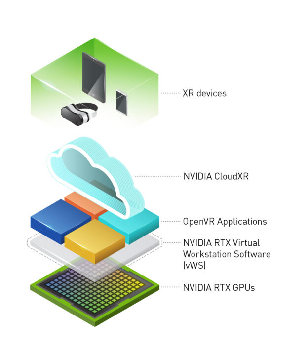
NVIDIA CloudXR Release 2.0 is now available. With NVIDIA CloudXR, users don’t need to be physically tethered to a high-performance computer to drive rich, immersive environments. The CloudXR SDK runs on NVIDIA servers located in the cloud, edge or on-premises, delivering the advanced graphics performance needed for wireless virtual, augmented or mixed reality environments — collectively known as XR.
This latest release includes new features that allow more client support for various devices, including Oculus Quest 2, HoloLens 2 Display, for AR streaming. And the new latency profiler helps providers and developers understand CloudXR latencies and performance.
Additional features include:
- Oculus Quest 2 Client support
- Oculus Quest and Oculus Quest 2 Link Support with Windows client
- HoloLens 2 display support with hand gestures mapped to controller buttons for interaction
- Foveated Scaling, which allows improved visual quality optimized to match HMD optics
- CloudXR Latency Profiler, which illustrates various latencies associated with the CloudXR streaming pipeline
- Android client ARM-64-v8 support for both AR and VR client
- Configurable log file size and removal
- Various bug fixes
Companies that have access to 5G networks can use NVIDIA CloudXR to stream immersive environments from their on-prem data centers. Telcos, software makers and device manufacturers can use the high bandwidth and low latency of 5G signals to provide high framerate, low-latency immersive XR experiences to millions of customers in more locations than previously possible.
“Using NVIDIA CloudXR and NVIDIA vGPU we have built a number of on-prem, high-performance solutions for customers who require the highest quality streaming XR,” said Andy Bowker, co-founder and CEO at The Grid Factory. “The NVIDIA CloudXR SDK has become a lynchpin for our end-to-end solutions, allowing us to deliver the highest quality turnkey solutions, and allowing our customers in turn to focus on their work instead of worrying about the technology.”
“NVIDIA CloudXR is an exciting new technology that’s becoming available on all platforms and devices,” said Greg Demchak, Director of the iLAB at Bentley. “With CloudXR, our customers will be able to extend their iTwin (Digital Twin) solutions to AR, VR, and MR devices.”
NVIDIA CloudXR Release 2.0 is now available for early access users. If you are interested in applying for access to this private beta, apply at the NVIDIA CloudXR DevZone Page.
To learn more about The Grid Factory and their CloudXR deployments, sign up for the upcoming webinar taking place on February 18.

 In this video, NVIDIA’s Alexey Panteleev explains the key details needed to add performant resampling to modern game engines. He also discusses roadmap plans for the recently announced RTXDI SDK.