Categories
Offsites

Google at ICML 2023

Groups across Google actively pursue research in the field of machine learning (ML), ranging from theory and application. We build ML systems to solve deep scientific and engineering challenges in areas of language, music, visual processing, algorithm development, and more. We aim to build a more collaborative ecosystem with the broader ML research community through open-sourcing tools and datasets, publishing our work, and actively participating in conferences.

Google is proud to be a Diamond Sponsor of the 40th International Conference on Machine Learning (ICML 2023), a premier annual conference, which is being held this week in Honolulu, Hawaii. As a leader in ML research, Google has a strong presence at this year’s conference with over 120 accepted papers and active involvement in a number of workshops and tutorials. Google is also proud to be a Platinum Sponsor for both the LatinX in AI and Women in Machine Learning workshops. We look forward to sharing some of our extensive ML research and expanding our partnership with the broader ML research community.

Registered for ICML 2023? We hope you’ll visit the Google booth to learn more about the exciting work, creativity, and fun that goes into solving a portion of the field’s most interesting challenges. Visit the @GoogleAI Twitter account to find out about Google booth activities (e.g., demos and Q&A sessions). See Google DeepMind’s blog to learn about their technical participation at ICML 2023.

Take a look below to learn more about the Google research being presented at ICML 2023 (Google affiliations in bold).

Board and Organizing Committee

Board Members include: Corinna Cortes, Hugo Larochelle

Tutorial Chairs include: Hanie Sedghi

Google Research booth activities

Presenters: Bryan Perozzi, Anton Tsitsulin, Brandon Mayer

Title: Unsupervised Graph Embedding @ Google (paper, EXPO workshop)

Tuesday, July 25th at 10:30 AM HST

Presenters: Zheng Xu

Title: Federated Learning of Gboard Language Models with Differential Privacy (paper 1, paper 2, blog post)

Tuesday, July 25th at 3:30 PM HST

Presenters: Thomas Kipf

Title: Self-supervised scene understanding (paper 1, paper 2)

Wednesday, July 26th at 10:30 AM HST

Presenters: Johannes von Oswald, Max Vladymyrov

Title: Transformers learn in-context by gradient descent (paper)

Wednesday, July 26th at 3:30 PM HST

Accepted papers

Scaling Vision Transformers to 22 Billion Parameters (see blog post)

Mostafa Dehghani, Josip Djolonga, Basil Mustafa, Piotr Padlewski, Jonathan Heek, Justin Gilmer, Andreas Steiner, Mathilde Caron, Robert Geirhos, Ibrahim Alabdulmohsin, Rodolphe Jenatton, Lucas Beyer, Michael Tschannen, Anurag Arnab, Xiao Wang, Carlos Riquelme, Matthias Minderer, Joan Puigcerver, Utku Evci, Manoj Kumar, Sjoerd van Steenkiste, Gamaleldin F. Elsayed, Aravindh Mahendran, Fisher Yu, Avital Oliver, Fantine Huot, Jasmijn Bastings, Mark Patrick Collier, Alexey Gritsenko, Vighnesh Birodkar, Cristina Vasconcelos, Yi Tay, Thomas Mensink, Alexander Kolesnikov, Filip Pavetić, Dustin Tran, Thomas Kipf, Mario Lučić, Xiaohua Zhai, Daniel Keysers, Jeremiah Harmsen, Neil Houlsby

Fast Inference from Transformers via Speculative Decoding

Yaniv Leviathan, Matan Kalman, Yossi Matias

Best of Both Worlds Policy Optimization

Christoph Dann, Chen-Yu Wei, Julian Zimmert

Inflow, Outflow, and Reciprocity in Machine Learning

Mukund Sundararajan, Walid Krichene

Transformers Learn In-Context by Gradient Descent

Johannes von Oswald, Eyvind Niklasson, Ettore Randazzo, João Sacramento, Alexander Mordvintsev, Andrey Zhmoginov, Max Vladymyrov

Arithmetic Sampling: Parallel Diverse Decoding for Large Language Models

Luke Vilnis, Yury Zemlyanskiy, Patrick Murray*, Alexandre Passos*, Sumit Sanghai

Differentially Private Hierarchical Clustering with Provable Approximation Guarantees (see blog post)

Jacob Imola*, Alessandro Epasto, Mohammad Mahdian, Vincent Cohen-Addad, Vahab Mirrokni

Multi-Epoch Matrix Factorization Mechanisms for Private Machine Learning

Christopher A. Choquette-Choo, H. Brendan McMahan, Keith Rush, Abhradeep Thakurta

Random Classification Noise Does Not Defeat All Convex Potential Boosters Irrespective of Model Choice

Yishay Mansour, Richard Nock, Robert Williamson

Simplex Random Features

Isaac Reid, Krzysztof Choromanski, Valerii Likhosherstov, Adrian Weller

Pix2Struct: Screenshot Parsing as Pretraining for Visual Language Understanding

Kenton Lee, Mandar Joshi, Iulia Turc, Hexiang Hu, Fangyu Liu, Julian Eisenschlos, Urvashi Khandelwal, Peter Shaw, Ming-Wei Chang, Kristina Toutanova

Mu2SLAM: Multitask, Multilingual Speech and Language Models

Yong Cheng, Yu Zhang, Melvin Johnson, Wolfgang Macherey, Ankur Bapna

Robust Budget Pacing with a Single Sample

Santiago Balseiro, Rachitesh Kumar*, Vahab Mirrokni, Balasubramanian Sivan, Di Wang

A Statistical Perspective on Retrieval-Based Models

Soumya Basu, Ankit Singh Rawat, Manzil Zaheer

Approximately Optimal Core Shapes for Tensor Decompositions

Mehrdad Ghadiri, Matthew Fahrbach, Gang Fu, Vahab Mirrokni

Efficient List-Decodable Regression Using Batches

Abhimanyu Das, Ayush Jain*, Weihao Kong, Rajat Sen

Efficient Training of Language Models Using Few-Shot Learning

Sashank J. Reddi, Sobhan Miryoosefi, Stefani Karp, Shankar Krishnan, Satyen Kale, Seungyeon Kim, Sanjiv Kumar

Fully Dynamic Submodular Maximization Over Matroids

Paul Duetting, Federico Fusco, Silvio Lattanzi, Ashkan Norouzi-Fard, Morteza Zadimoghaddam

GFlowNet-EM for Learning Compositional Latent Variable Models

Edward J Hu, Nikolay Malkin, Moksh Jain, Katie Everett, Alexandros Graikos, Yoshua Bengio

Improved Online Learning Algorithms for CTR Prediction in Ad Auctions

Zhe Feng, Christopher Liaw, Zixin Zhou

Large Language Models Struggle to Learn Long-Tail Knowledge

Nikhil Kandpal, Haikang Deng, Adam Roberts, Eric Wallace, Colin Raffel

Multi-channel Autobidding with Budget and ROI Constraints

Yuan Deng, Negin Golrezaei, Patrick Jaillet, Jason Cheuk Nam Liang, Vahab Mirrokni

Multi-layer Neural Networks as Trainable Ladders of Hilbert Spaces

Zhengdao Chen

On User-Level Private Convex Optimization

Badih Ghazi, Pritish Kamath, Ravi Kumar, Raghu Meka, Pasin Manurangsi, Chiyuan Zhang

PAC Generalization via Invariant Representations

Advait U Parulekar, Karthikeyan Shanmugam, Sanjay Shakkottai

Regularization and Variance-Weighted Regression Achieves Minimax Optimality in Linear MDPs: Theory and Practice

Toshinori Kitamura, Tadashi Kozuno, Yunhao Tang, Nino Vieillard, Michal Valko, Wenhao Yang, Jincheng Mei, Pierre Menard, Mohammad Gheshlaghi Azar, Remi Munos, Olivier Pietquin, Matthieu Geist,Csaba Szepesvari, Wataru Kumagai, Yutaka Matsuo

Speeding Up Bellman Ford via Minimum Violation Permutations

Silvio Lattanzi, Ola Svensson, Sergei Vassilvitskii

Statistical Indistinguishability of Learning Algorithms

Alkis Kalavasis, Amin Karbasi, Shay Moran, Grigoris Velegkas

Test-Time Adaptation with Slot-Centric Models

Mihir Prabhudesai, Anirudh Goyal, Sujoy Paul, Sjoerd van Steenkiste, Mehdi S. M. Sajjadi, Gaurav Aggarwal, Thomas Kipf, Deepak Pathak, Katerina Fragkiadaki>

Algorithms for Bounding Contribution for Histogram Estimation Under User-Level Privacy

Yuhan Liu*, Ananda Theertha Suresh, Wennan Zhu, Peter Kairouz, Marco Gruteser

Bandit Online Linear Optimization with Hints and Queries

Aditya Bhaskara, Ashok Cutkosky, Ravi Kumar, Manish Purohit

CLUTR: Curriculum Learning via Unsupervised Task Representation Learning

Abdus Salam Azad, Izzeddin Gur, Jasper Emhoff, Nathaniel Alexis, Aleksandra Faust, Pieter Abbeel, Ion Stoica

CSP: Self-Supervised Contrastive Spatial Pre-training for Geospatial-Visual Representations

Gengchen Mai, Ni Lao, Yutong He, Jiaming Song, Stefano Ermon

Ewald-Based Long-Range Message Passing for Molecular Graphs

Arthur Kosmala, Johannes Gasteiger, Nicholas Gao, Stephan Günnemann

Fast (1+ε)-Approximation Algorithms for Binary Matrix Factorization

Ameya Velingker, Maximilian Vötsch, David Woodruff, Samson Zhou

Federated Linear Contextual Bandits with User-Level Differential Privacy

Ruiquan Huang, Huanyu Zhang, Luca Melis, Milan Shen, Meisam Hejazinia, Jing Yang

Investigating the Role of Model-Based Learning in Exploration and Transfer

Jacob C Walker, Eszter Vértes, Yazhe Li, Gabriel Dulac-Arnold, Ankesh Anand, Theophane Weber, Jessica B Hamrick

Label Differential Privacy and Private Training Data Release

Robert Busa-Fekete, Andres Munoz, Umar Syed, Sergei Vassilvitskii

Lifelong Language Pretraining with Distribution-Specialized Experts

Wuyang Chen*, Yanqi Zhou, Nan Du, Yanping Huang, James Laudon, Zhifeng Chen, Claire Cui

Multi-User Reinforcement Learning with Low Rank Rewards

Dheeraj Mysore Nagaraj, Suhas S Kowshik, Naman Agarwal, Praneeth Netrapalli, Prateek Jain

Multi-View Masked World Models for Visual Robotic Manipulation

Younggyo Seo, Junsu Kim, Stephen James, Kimin Lee, Jinwoo Shin, Pieter Abbeel

PaLM-E: An Embodied Multimodal Language Model (see blog post)

Danny Driess, Fei Xia, Mehdi S. M. Sajjadi, Corey Lynch, Aakanksha Chowdhery, Brian Ichter,Ayzaan Wahid, Jonathan Tompson, Quan Vuong, Tianhe Yu, Wenlong Huang, Yevgen Chebotar, Pierre Sermanet, Daniel Duckworth, Sergey Levine, Vincent Vanhoucke, Karol Hausman, Marc Toussaint, Klaus Greff, Andy Zeng, Igor Mordatch, Pete Florence

Private Federated Learning with Autotuned Compression

Enayat Ullah*, Christopher A. Choquette-Choo, Peter Kairouz, Sewoong Oh

Refined Regret for Adversarial MDPs with Linear Function Approximation

Yan Dai, Haipeng Luo, Chen-Yu Wei, Julian Zimmert

Scaling Up Dataset Distillation to ImageNet-1K with Constant Memory

Justin Cui, Ruoche Wan, Si Si, Cho-Jui Hsieh

SGD with AdaGrad Stepsizes: Full Adaptivity with High Probability to Unknown Parameters, Unbounded Gradients and Affine Variance

Amit Attia, Tomer Koren

The Statistical Benefits of Quantile Temporal-Difference Learning for Value Estimation

Mark Rowland, Yunhao Tang, Clare Lyle, Rémi Munos, Marc G. Bellemare, Will Dabney

Unveiling The Mask of Position-Information Pattern Through the Mist of Image Features

Chieh Hubert Lin, Hung-Yu Tseng, Hsin-Ying Lee, Maneesh Kumar Singh, Ming-Hsuan Yang

User-Level Private Stochastic Convex Optimization with Optimal Rates

Raef Bassily, Ziteng Sun

A Simple Zero-Shot Prompt Weighting Technique to Improve Prompt Ensembling in Text-Image Models

James Urquhart Allingham*, Jie Ren, Michael W Dusenberry, Xiuye Gu, Yin Cui, Dustin Tran, Jeremiah Zhe Liu, Balaji Lakshminarayanan

Can Large Language Models Reason About Program Invariants?

Kexin Pei, David Bieber, Kensen Shi, Charles Sutton, Pengcheng Yin

Concurrent Shuffle Differential Privacy Under Continual Observation

Jay Tenenbaum, Haim Kaplan, Yishay Mansour, Uri Stemmer

Constant Matters: Fine-Grained Error Bound on Differentially Private Continual Observation

Hendrik Fichtenberger, Monika Henzinger, Jalaj Upadhyay

Cross-Entropy Loss Functions: Theoretical Analysis and Applications

Anqi Mao, Mehryar Mohri, Yutao Zhong

Efficient Rate Optimal Regret for Adversarial Contextual MDPs Using Online Function Approximation

Orin Levy, Alon Cohen, Asaf Cassel, Yishay Mansour

Fairness in Streaming Submodular Maximization Over a Matroid Constraint

Marwa El Halabi, Federico Fusco, Ashkan Norouzi-Fard, Jakab Tardos, Jakub Tarnawski

The Flan Collection: Designing Data and Methods for Effective Instruction Tuning (see blog post)

Shayne Longpre, Le Hou, Tu Vu, Albert Webson, Hyung Won Chung, Yi Tay, Denny Zhou, Quoc V Le, Barret Zoph, Jason Wei, Adam Roberts

Graph Reinforcement Learning for Network Control via Bi-level Optimization

Daniele Gammelli, James Harrison, Kaidi Yang, Marco Pavone, Filipe Rodrigues, Francisco C. Pereira

Learning-Augmented Private Algorithms for Multiple Quantile Release

Mikhail Khodak*, Kareem Amin, Travis Dick, Sergei Vassilvitskii

LegendreTron: Uprising Proper Multiclass Loss Learning

Kevin H Lam, Christian Walder, Spiridon Penev, Richard Nock

Measuring the Impact of Programming Language Distribution

Gabriel Orlanski*, Kefan Xiao, Xavier Garcia, Jeffrey Hui, Joshua Howland, Jonathan Malmaud, Jacob Austin, Rishabh Singh, Michele Catasta*

Multi-task Differential Privacy Under Distribution Skew

Walid Krichene, Prateek Jain, Shuang Song, Mukund Sundararajan, Abhradeep Thakurta, Li Zhang

Muse: Text-to-Image Generation via Masked Generative Transformers

Huiwen Chang, Han Zhang, Jarred Barber, AJ Maschinot, José Lezama, Lu Jiang, Ming-Hsuan Yang, Kevin Murphy, William T. Freeman, Michael Rubinstein, Yuanzhen Li, Dilip Krishnan

On the Convergence of Federated Averaging with Cyclic Client Participation

Yae Jee Cho, Pranay Sharma, Gauri Joshi, Zheng Xu, Satyen Kale, Tong Zhang

Optimal Stochastic Non-smooth Non-convex Optimization Through Online-to-Non-convex Conversion

Ashok Cutkosky, Harsh Mehta, Francesco Orabona

Out-of-Domain Robustness via Targeted Augmentations

Irena Gao, Shiori Sagawa, Pang Wei Koh, Tatsunori Hashimoto, Percy Liang

Polynomial Time and Private Learning of Unbounded Gaussian Mixture Models

Jamil Arbas, Hassan Ashtiani, Christopher Liaw

Pre-computed Memory or On-the-Fly Encoding? A Hybrid Approach to Retrieval Augmentation Makes the Most of Your Compute

Michiel de Jong, Yury Zemlyanskiy, Nicholas FitzGerald, Joshua Ainslie, Sumit Sanghai, Fei Sha, William W. Cohen

Scalable Adaptive Computation for Iterative Generation

Allan Jabri*, David J. Fleet, Ting Chen

Scaling Spherical CNNs

Carlos Esteves, Jean-Jacques Slotine, Ameesh Makadia

STEP: Learning N:M Structured Sparsity Masks from Scratch with Precondition

Yucheng Lu, Shivani Agrawal, Suvinay Subramanian, Oleg Rybakov, Christopher De Sa, Amir Yazdanbakhsh

Stratified Adversarial Robustness with Rejection

Jiefeng Chen, Jayaram Raghuram, Jihye Choi, Xi Wu, Yingyu Liang, Somesh Jha

When Does Privileged information Explain Away Label Noise?

Guillermo Ortiz-Jimenez*, Mark Collier, Anant Nawalgaria, Alexander D’Amour, Jesse Berent, Rodolphe Jenatton, Effrosyni Kokiopoulou

Adaptive Computation with Elastic Input Sequence

Fuzhao Xue*, Valerii Likhosherstov, Anurag Arnab, Neil Houlsby, Mostafa Dehghani, Yang You

Can Neural Network Memorization Be Localized?

Pratyush Maini, Michael C. Mozer, Hanie Sedghi, Zachary C. Lipton, J. Zico Kolter, Chiyuan Zhang

Controllability-Aware Unsupervised Skill Discovery

Seohong Park, Kimin Lee, Youngwoon Lee, Pieter Abbeel

Efficient Learning of Mesh-Based Physical Simulation with Bi-Stride Multi-Scale Graph Neural Network

Yadi Cao, Menglei Chai, Minchen Li, Chenfanfu Jiang

Federated Heavy Hitter Recovery Under Linear Sketching

Adria Gascon, Peter Kairouz, Ziteng Sun, Ananda Theertha Suresh

Graph Generative Model for Benchmarking Graph Neural Networks

Minji Yoon, Yue Wu, John Palowitch, Bryan Perozzi, Russ Salakhutdinov

H-Consistency Bounds for Pairwise Misranking Loss Surrogates

Anqi Mao, Mehryar Mohri, Yutao Zhong

Improved Regret for Efficient Online Reinforcement Learning with Linear Function Approximation

Uri Sherman, Tomer Koren, Yishay Mansour

Invariant Slot Attention: Object Discovery with Slot-Centric Reference Frames

Ondrej Biza*, Sjoerd van Steenkiste, Mehdi S. M. Sajjadi, Gamaleldin Fathy Elsayed, Aravindh Mahendran, Thomas Kipf

Multi-task Off-Policy Learning from Bandit Feedback

Joey Hong, Branislav Kveton, Manzil Zaheer, Sumeet Katariya, Mohammad Ghavamzadeh

Optimal No-Regret Learning for One-Sided Lipschitz Functions

Paul Duetting, Guru Guruganesh, Jon Schneider, Joshua Ruizhi Wang

Policy Mirror Ascent for Efficient and Independent Learning in Mean Field Games

Batuhan Yardim, Semih Cayci, Matthieu Geist, Niao He

Regret Minimization and Convergence to Equilibria in General-Sum Markov Games

Liad Erez, Tal Lancewicki, Uri Sherman, Tomer Koren, Yishay Mansour

Reinforcement Learning Can Be More Efficient with Multiple Rewards

Christoph Dann, Yishay Mansour, Mehryar Mohri

Reinforcement Learning with History-Dependent Dynamic Contexts

Guy Tennenholtz, Nadav Merlis, Lior Shani, Martin Mladenov, Craig Boutlier

User-Defined Event Sampling and Uncertainty Quantification in Diffusion Models for Physical Dynamical Systems

Marc Anton Finzi*, Anudhyan Boral, Andrew Gordon Wilson, Fei Sha, Leonardo Zepeda-Nunez

Discrete Key-Value Bottleneck

Frederik Träuble, Anirudh Goyal, Nasim Rahaman, Michael Curtis Mozer, Kenji Kawaguchi, Yoshua Bengio, Bernhard Schölkopf

DSGD-CECA: Decentralized SGD with Communication-Optimal Exact Consensus Algorithm

Lisang Ding, Kexin Jin, Bicheng Ying, Kun Yuan, Wotao Yin

Exphormer: Sparse Transformers for Graphs

Hamed Shirzad, Ameya Velingker, Balaji Venkatachalam, Danica J. Sutherland, Ali Kemal Sinop

Fast, Differentiable and Sparse Top-k: A Convex Analysis Perspective

Michael Eli Sander*, Joan Puigcerver, Josip Djolonga, Gabriel Peyré, Mathieu Blondel

Improved Policy Evaluation for Randomized Trials of Algorithmic Resource Allocation

Aditya Mate, Bryan Wilder, Aparna Taneja, Milind Tambe

In Search for a Generalizable Method for Source Free Domain Adaptation

Malik Boudiaf*, Tom Denton, Bart van Merrienboer, Vincent Dumoulin, Eleni Triantafillou

Learning Rate Schedules in the Presence of Distribution Shift

Matthew Fahrbach, Adel Javanmard, Vahab Mirrokni, Pratik Worah

Not All Semantics Are Created Equal: Contrastive Self-Supervised Learning with Automatic Temperature Individualization

Zi-Hao Qiu, Quanqi Hu, Zhuoning Yuan, Denny Zhou, Lijun Zhang, Tianbao Yang

On the Relationship Between Explanation and Prediction: A Causal View

Amir-Hossein Karimi*, Krikamol Muandet, Simon Kornblith, Bernhard Schölkopf, Been Kim

On the Role of Attention in Prompt-Tuning

Samet Oymak, Ankit Singh Rawat, Mahdi Soltanolkotabi, Christos Thrampoulidis

PLay: Parametrically Conditioned Layout Generation Using Latent Diffusion

Chin-Yi Cheng, Forrest Huang, Gang Li, Yang Li

The Power of Learned Locally Linear Models for Nonlinear Policy Optimization

Daniel Pfrommer, Max Simchowitz, Tyler Westenbroek, Nikolai Matni, Stephen Tu

Relevant Walk Search for Explaining Graph Neural Networks

Ping Xiong, Thomas Schnake, Michael Gastegger, Grégoire Montavon, Klaus Robert Muller,Shinichi Nakajima

Repository-Level Prompt Generation for Large Language Models of Code

Disha Shrivastava, Hugo Larochelle, Daniel Tarlow

Robust and Private Stochastic Linear Bandits

Vasileios Charisopoulos*, Hossein Esfandiari, Vahab Mirrokni

Simple Diffusion: End-to-End Diffusion for High Resolution Images

Emiel Hoogeboom, Jonathan Heek, Tim Salimans

Tied-Augment: Controlling Representation Similarity Improves Data Augmentation

Emirhan Kurtulus, Zichao Li, Yann Dauphin, Ekin D. Cubuk

Why Is Public Pre-Training Necessary for Private Model Training?

Arun Ganesh, Mahdi Haghifam*, Milad Nasr, Sewoong Oh, Thomas Steinke, Om Thakkar, Abhradeep Guha Thakurta, Lun Wang

A Connection Between One-Step RL and Critic Regularization in Reinforcement Learning

Benjamin Eysenbach, Matthieu Geist, Sergey Levine, Ruslan Salakhutdinov

Beyond Uniform Lipschitz Condition in Differentially Private Optimization

Rudrajit Das*, Satyen Kale, Zheng Xu, Tong Zhang, Sujay Sanghavi

Efficient Graph Field Integrators Meet Point Clouds

Krzysztof Choromanski, Arijit Sehanobish, Han Lin, Yunfan Zhao, Eli Berger, Tetiana Parshakova, Alvin Pan, David Watkins, Tianyi Zhang, Valerii Likhosherstov, Somnath Basu Roy Chowdhury, Avinava Dubey, Deepali Jain, Tamas Sarlos, Snigdha Chaturvedi, Adrian Weller

Fast as CHITA: Neural Network Pruning with Combinatorial Optimization

Riade Benbaki, Wenyu Chen, Xiang Meng, Hussein Hazimeh, Natalia Ponomareva, Zhe Zhao, Rahul Mazumder

Jump-Start Reinforcement Learning (see blog post)

Ikechukwu Uchendu*, Ted Xiao, Yao Lu, Banghua Zhu, Mengyuan Yan, Joséphine Simon, Matthew Bennice, Chuyuan Fu, Cong Ma, Jiantao Jiao, Sergey Levine, Karol Hausman

Learning in POMDPs is Sample-Efficient with Hindsight Observability

Jonathan Lee, Alekh Agarwal, Christoph Dann, Tong Zhang

Low-Variance Gradient Estimation in Unrolled Computation Graphs with ES-Single

Paul Vicol

Masked Trajectory Models for Prediction, Representation, and Control

Philipp Wu, Arjun Majumdar, Kevin Stone, Yixin Lin, Igor Mordatch, Pieter Abbeel, Aravind Rajeswaran

Overcoming Simplicity Bias in Deep Networks Using a Feature Sieve

Rishabh Tiwari, Pradeep Shenoy

Pairwise Ranking Losses of Click-Through Rates Prediction for Welfare Maximization in Ad Auctions

Boxiang Lyu, Zhe Feng, Zachary Robertson, Sanmi Koyejo

Predictive Flows for Faster Ford-Fulkerson

Sami Davies, Benjamin Moseley, Sergei Vassilvitskii, Yuyan Wang

Scaling Laws for Multilingual Neural Machine Translation

Patrick Fernandes, Behrooz Ghorbani, Xavier Garcia, Markus Freitag, Orhan Firat

Sequential Monte Carlo Learning for Time Series Structure Discovery

Feras Saad, Brian Patton, Matthew Douglas Hoffman, Rif A. Saurous, Vikash Mansinghka

Stochastic Gradient Succeeds for Bandits

Jincheng Mei, Zixin Zhong, Bo Dai, Alekh Agarwal, Csaba Szepesvari, Dale Schuurmans

Subset-Based Instance Optimality in Private Estimation

Travis Dick, Alex Kulesza, Ziteng Sun, Ananda Theertha Suresh

The Unreasonable Effectiveness of Few-Shot Learning for Machine Translation

Xavier Garcia, Yamini Bansal, Colin Cherry, George Foster, Maxim Krikun, Melvin Johnson, Orhan Firat

Tutorials

Self-Supervised Learning in Vision: from Research Advances to Best Practices

Xinlei Chen, Ishan Misra, Randall Balestriero, Mathilde Caron, Christoph Feichtenhofer, Mark Ibrahim

How to DP-fy ML: A Practical Tutorial to Machine Learning with Differential Privacy (see blog post)

Sergei Vassilvitskii, Natalia Ponomareva, Zheng Xu

Recent Advances in the Generalization Theory of Neural Networks

Tengyu Ma, Alex Damian

EXPO Day workshops

Graph Neural Networks in Tensorflow: A Practical Guide

Workshop Organizers include: Bryan Perozzi, Anton Tsitsulin, Brandon Mayer, Jonathan Halcrow

Google sponsored affinity workshops

LatinX in AI (LAXAI)

Platinum Sponsor

Keynote Speaker: Monica Ribero

Panelist: Yao Qin

Women in Machine Learning (WiML)

Platinum Sponsor

Panelists: Yao Qin

Workshops

Federated Learning and Analytics in Practice: Algorithms, Systems, Applications, and Opportunities

Organizer: Peter Kairouz, Zheng Xu

Speaker: Brendan McMahan

Interpretable Machine Learning in Healthcare (IMLH)

Organizer: Ramin Zabih

Knowledge and Logical Reasoning in the Era of Data-Driven Learning

Organizer: Beliz Günel

The Many Facets of Preference-Based Learning (MFPL)

Organizer: Robert Busa-Fekete, Mohammad Ghavamzadeh

The Synergy of Scientific and Machine Learning Modelling (SynS & ML)

Speaker: Sercan Arik

Theory of Mind in Communicating Agents

Organizer: Pei Zhou

Artificial Intelligence & Human Computer Interaction

Organizer: Yang Li, Forrest Huang

Data-Centric Machine Learning Research (DMLR)

Organizer: Alicia Parrish, Najoung Kim

Speaker: Peter Mattson

Neural Compression: from Information Theory to Applications

Speaker: Johannes Ballé

Panelist: George Toderici

Neural Conversational AI Workshop – What’s Left to TEACH (Trustworthy, Enhanced, Adaptable, Capable and Human-centric) Chatbots?

Organizer: Ahmad Beirami

Spurious Correlations, Invariance and Stability (SCIS)

Organizer: Amir Feder


* Work done while at Google

Categories
Offsites

Using societal context knowledge to foster the responsible application of AI

AI-related products and technologies are constructed and deployed in a societal context: that is, a dynamic and complex collection of social, cultural, historical, political and economic circumstances. Because societal contexts by nature are dynamic, complex, non-linear, contested, subjective, and highly qualitative, they are challenging to translate into the quantitative representations, methods, and practices that dominate standard machine learning (ML) approaches and responsible AI product development practices.

The first phase of AI product development is problem understanding, and this phase has tremendous influence over how problems (e.g., increasing cancer screening availability and accuracy) are formulated for ML systems to solve as well many other downstream decisions, such as dataset and ML architecture choice. When the societal context in which a product will operate is not articulated well enough to result in robust problem understanding, the resulting ML solutions can be fragile and even propagate unfair biases.

When AI product developers lack access to the knowledge and tools necessary to effectively understand and consider societal context during development, they tend to abstract it away. This abstraction leaves them with a shallow, quantitative understanding of the problems they seek to solve, while product users and society stakeholders — who are proximate to these problems and embedded in related societal contexts — tend to have a deep qualitative understanding of those same problems. This qualitative–quantitative divergence in ways of understanding complex problems that separates product users and society from developers is what we call the problem understanding chasm.

This chasm has repercussions in the real world: for example, it was the root cause of racial bias discovered by a widely used healthcare algorithm intended to solve the problem of choosing patients with the most complex healthcare needs for special programs. Incomplete understanding of the societal context in which the algorithm would operate led system designers to form incorrect and oversimplified causal theories about what the key problem factors were. Critical socio-structural factors, including lack of access to healthcare, lack of trust in the health care system, and underdiagnosis due to human bias, were left out while spending on healthcare was highlighted as a predictor of complex health need.

To bridge the problem understanding chasm responsibly, AI product developers need tools that put community-validated and structured knowledge of societal context about complex societal problems at their fingertips — starting with problem understanding, but also throughout the product development lifecycle. To that end, Societal Context Understanding Tools and Solutions (SCOUTS) — part of the Responsible AI and Human-Centered Technology (RAI-HCT) team within Google Research — is a dedicated research team focused on the mission to “empower people with the scalable, trustworthy societal context knowledge required to realize responsible, robust AI and solve the world’s most complex societal problems.” SCOUTS is motivated by the significant challenge of articulating societal context, and it conducts innovative foundational and applied research to produce structured societal context knowledge and to integrate it into all phases of the AI-related product development lifecycle. Last year we announced that Jigsaw, Google’s incubator for building technology that explores solutions to threats to open societies, leveraged our structured societal context knowledge approach during the data preparation and evaluation phases of model development to scale bias mitigation for their widely used Perspective API toxicity classifier. Going forward SCOUTS’ research agenda focuses on the problem understanding phase of AI-related product development with the goal of bridging the problem understanding chasm.

Bridging the AI problem understanding chasm

Bridging the AI problem understanding chasm requires two key ingredients: 1) a reference frame for organizing structured societal context knowledge and 2) participatory, non-extractive methods to elicit community expertise about complex problems and represent it as structured knowledge. SCOUTS has published innovative research in both areas.

An illustration of the problem understanding chasm.

A societal context reference frame

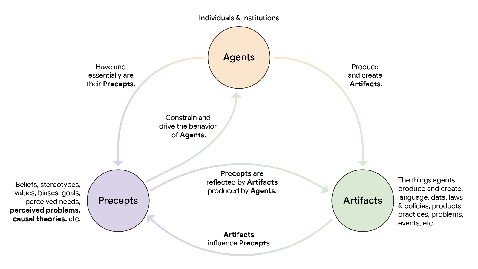
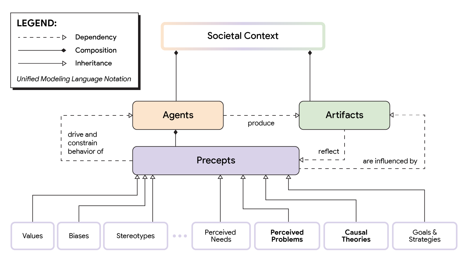
An essential ingredient for producing structured knowledge is a taxonomy for creating the structure to organize it. SCOUTS collaborated with other RAI-HCT teams (TasC, Impact Lab), Google DeepMind, and external system dynamics experts to develop a taxonomic reference frame for societal context. To contend with the complex, dynamic, and adaptive nature of societal context, we leverage complex adaptive systems (CAS) theory to propose a high-level taxonomic model for organizing societal context knowledge. The model pinpoints three key elements of societal context and the dynamic feedback loops that bind them together: agents, precepts, and artifacts.

  • Agents: These can be individuals or institutions.
  • Precepts: The preconceptions — including beliefs, values, stereotypes and biases — that constrain and drive the behavior of agents. An example of a basic precept is that “all basketball players are over 6 feet tall.” That limiting assumption can lead to failures in identifying basketball players of smaller stature.
  • Artifacts: Agent behaviors produce many kinds of artifacts, including language, data, technologies, societal problems and products.

The relationships between these entities are dynamic and complex. Our work hypothesizes that precepts are the most critical element of societal context and we highlight the problems people perceive and the causal theories they hold about why those problems exist as particularly influential precepts that are core to understanding societal context. For example, in the case of racial bias in a medical algorithm described earlier, the causal theory precept held by designers was that complex health problems would cause healthcare expenditures to go up for all populations. That incorrect precept directly led to the choice of healthcare spending as the proxy variable for the model to predict complex healthcare need, which in turn led to the model being biased against Black patients who, due to societal factors such as lack of access to healthcare and underdiagnosis due to bias on average, do not always spend more on healthcare when they have complex healthcare needs. A key open question is how can we ethically and equitably elicit causal theories from the people and communities who are most proximate to problems of inequity and transform them into useful structured knowledge?

Illustrative version of societal context reference frame.
Taxonomic version of societal context reference frame.

Working with communities to foster the responsible application of AI to healthcare

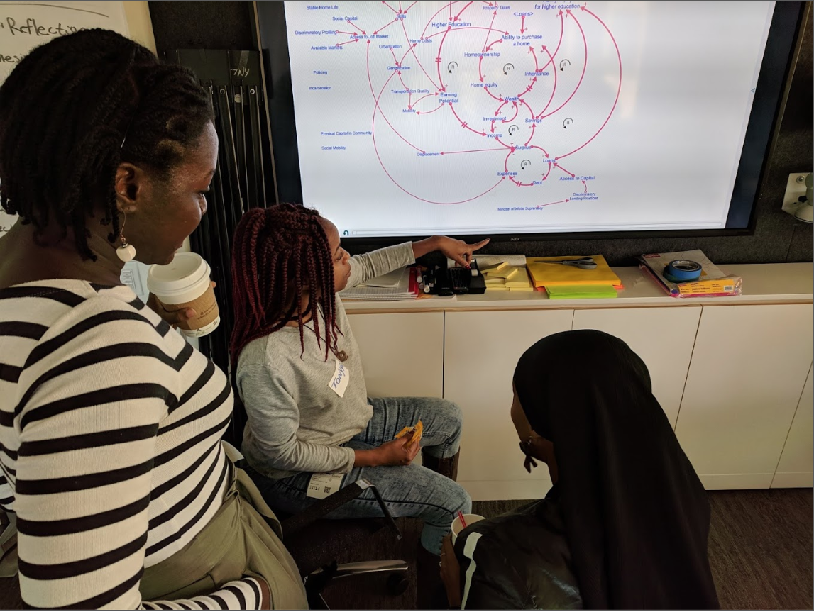
Since its inception, SCOUTS has worked to build capacity in historically marginalized communities to articulate the broader societal context of the complex problems that matter to them using a practice called community based system dynamics (CBSD). System dynamics (SD) is a methodology for articulating causal theories about complex problems, both qualitatively as causal loop and stock and flow diagrams (CLDs and SFDs, respectively) and quantitatively as simulation models. The inherent support of visual qualitative tools, quantitative methods, and collaborative model building makes it an ideal ingredient for bridging the problem understanding chasm. CBSD is a community-based, participatory variant of SD specifically focused on building capacity within communities to collaboratively describe and model the problems they face as causal theories, directly without intermediaries. With CBSD we’ve witnessed community groups learn the basics and begin drawing CLDs within 2 hours.

Data 4 Black Lives community members learning system dynamics.

There is a huge potential for AI to improve medical diagnosis. But the safety, equity, and reliability of AI-related health diagnostic algorithms depends on diverse and balanced training datasets. An open challenge in the health diagnostic space is the dearth of training sample data from historically marginalized groups. SCOUTS collaborated with the Data 4 Black Lives community and CBSD experts to produce qualitative and quantitative causal theories for the data gap problem. The theories include critical factors that make up the broader societal context surrounding health diagnostics, including cultural memory of death and trust in medical care.

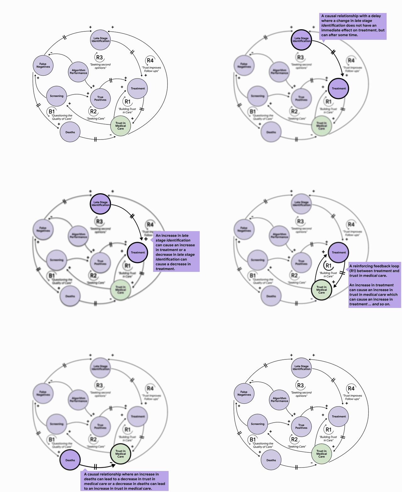
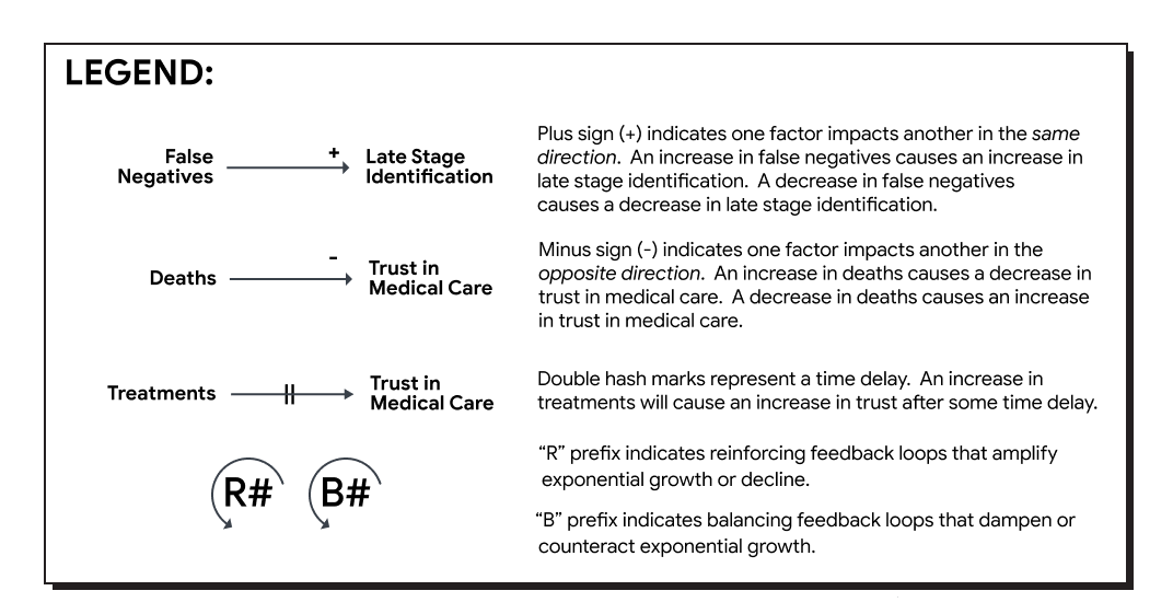
The figure below depicts the causal theory generated during the collaboration described above as a CLD. It hypothesizes that trust in medical care influences all parts of this complex system and is the key lever for increasing screening, which in turn generates data to overcome the data diversity gap.

Causal loop diagram of the health diagnostics data gap

These community-sourced causal theories are a first step to bridge the problem understanding chasm with trustworthy societal context knowledge.

Conclusion

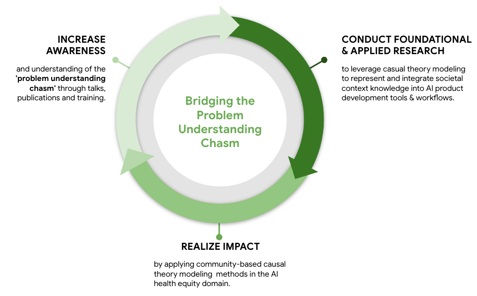
As discussed in this blog, the problem understanding chasm is a critical open challenge in responsible AI. SCOUTS conducts exploratory and applied research in collaboration with other teams within Google Research, external community, and academic partners across multiple disciplines to make meaningful progress solving it. Going forward our work will focus on three key elements, guided by our AI Principles:

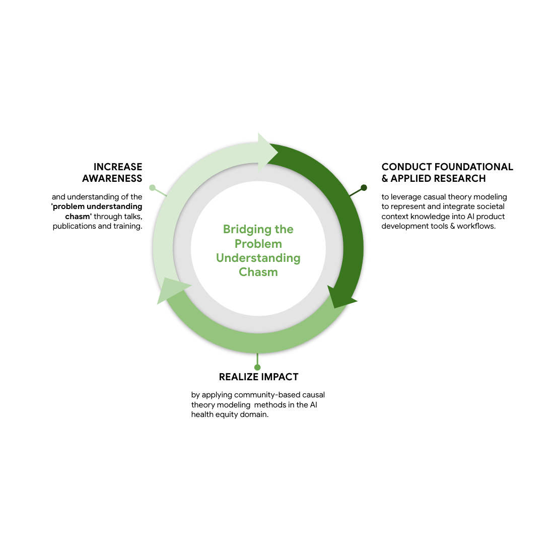
  1. Increase awareness and understanding of the problem understanding chasm and its implications through talks, publications, and training.
  2. Conduct foundational and applied research for representing and integrating societal context knowledge into AI product development tools and workflows, from conception to monitoring, evaluation and adaptation.
  3. Apply community-based causal modeling methods to the AI health equity domain to realize impact and build society’s and Google’s capability to produce and leverage global-scale societal context knowledge to realize responsible AI.
SCOUTS flywheel for bridging the problem understanding chasm.

Acknowledgments

Thank you to John Guilyard for graphics development, everyone in SCOUTS, and all of our collaborators and sponsors.

Categories
Misc

A Comprehensive Guide on Interaction Terms in Time Series Forecasting

Modeling time series data can be challenging (and fascinating) due to its inherent complexity and unpredictability. Long-term trends in time series can change…
Modeling time series data can be challenging (and fascinating) due to its inherent complexity and unpredictability. Long-term trends in time series can change drastically due to certain events, for example. Recall the beginning of the global pandemic, when businesses such as airlines or brick-and-mortar shops saw a quick decline in the number of customers and sales. In contrast, e-commerce businesses continued to operate with less disruption.

Interaction terms can help model such patterns. They capture complex relationships between variables and, as a result, lead to more accurate predictions.

This post explores:

  • Interaction terms in the context of time series forecasting
  • Benefits of interaction terms when modeling complex relationships
  • How to effectively implement interaction terms in your models 

Overview of interaction terms

Interaction terms enable you to investigate whether the relationship between the target and a feature changes depending on the value of another feature. For more details, see my previous post, A Comprehensive Guide to Interaction Terms in Linear Regression.

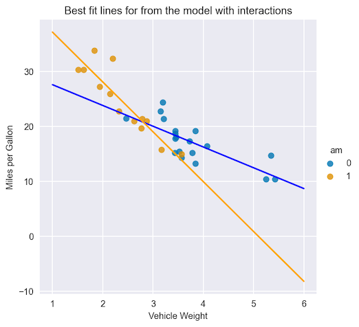
Figure 1 shows a scatterplot that represents the relationship between miles per gallon (target) and the weight of a vehicle (feature). The relationship is quite different depending on the transmission type (another feature).

Line plot showing the best fit lines for vehicle transmission types. They clearly have different slopes.
Figure 1. Best fit lines for vehicle transmission type, including interaction terms

Improving linear model accuracy

Without using interaction terms, a linear model would not be able to capture such a complex relationship. Effectively, it would assign the same coefficient for the weight feature, regardless of the type of transmission. Figure 1 shows the coefficients (slope of the line) by weight feature, which are drastically different for different transmission types.

To overcome this fallacy and make the linear model more flexible, add interaction terms. In general, they are a multiplication of the original features. By adding these new variables to the regression model, you can measure the effects of the interaction between them and the target. 

Interaction terms in time series forecasting

Interaction terms make linear models more flexible. The following example shows how they work in the context of time series forecasting.

Prerequisites

First, load the required libraries:

import numpy as np
import pandas as pd

from sklearn.linear_model import LinearRegression

import seaborn as sns
import matplotlib.pyplot as plt

Dataset generation

Then, generate some artificial time series data with the following characteristics:

  • 10 years of daily data
  • Repeating patterns (seasonality) present in the time series
  • A decreasing trend over the first 7 years
  • No trend in the last 3 years
  • Random noise, added as the last step
# for reproducibility
np.random.seed(42)

# generate the DataFrame with dates
range_of_dates = pd.date_range(
   start="2010-01-01",
   end="2019-12-30"
)
df = pd.DataFrame(index=range_of_dates)

# create a sequence of day numbers
df["linear_trend"] = range(len(df))
df["trend"] = 0.004 * df["linear_trend"].values[::-1]
df.loc["2017-01-01":, "trend"] = 4

# generate the components of the target
signal_1 = 10 + 4 * np.sin(df["linear_trend"] / 365 * 2 * np.pi)
noise = np.random.normal(0, 0.85, len(df))

# combine them to get the target series
df["target"] = signal_1 + noise + df["trend"]

# plot
df["target"].plot(title="Generated time series");

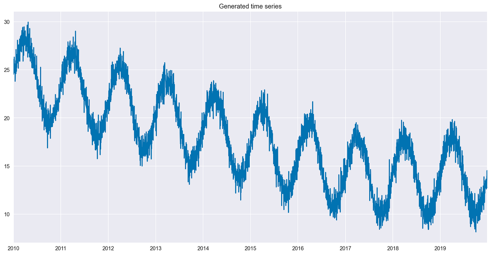
Figure 2 shows the generated time series, which includes all the desired characteristics.

A time series plot including all the desired characteristics, with a slight downward trend over time and containing multiple increases and decreases
Figure 2. The generated time series

Training the benchmark model

Now train a linear model and inspect the best fit line. For this step, create very simple models with a few features. This enables you to visually inspect the impact of the interaction term on the model’s fit.

The simplest model possible contains one feature — an indicator of the passage of time. The linear_trend column created for the time series is effectively the row number of the DataFrame (ordered by date).

X = df[["linear_trend"]]
y = df[["target"]]

lm = LinearRegression()
lm.fit(X, y)

df["model_1"] = lm.predict(X)

df[["target", "model_1"]].plot(title="Linear trend");

It is worth mentioning that the point is not to properly evaluate the forecasts using separate train and test sets, but rather to explain the impact of the interaction terms on the model’s fit. It is easier to observe the interaction term’s impact by inspecting the fitted values (prediction on the training set) and comparing those fitted values to the original time series. 

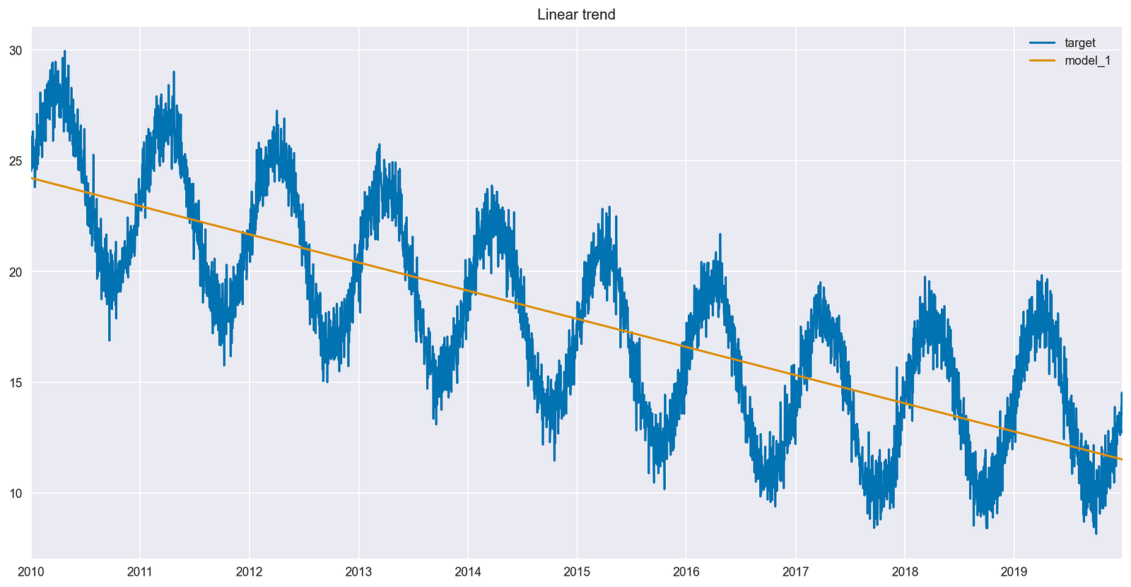
Figure 3 shows that the linear model identified a decreasing trend for the entire time series. At the same time, the fit seems off for the last 3 years of data, as there is no trend there.

The plot shows that the fitted line is the same for the entire dataset, thus not capturing the pattern change in the last 3 years.
Figure 3. Best fit line obtained from a linear model using linear trend as a feature

Add a breakpoint

Next, try to make the model learn the new pattern (trend change) using feature engineering. To do so, create a breakpoint, which is a placeholder variable indicating whether a given observation is after January 1, 2017. In this case, the exact point in time when the trend change happened is known. 

Next, train another linear model, this time with two features:

df["after_2017_breakpoint"] = np.where(df.index >= pd.Timestamp('2017-01-01'), 1, 0)

X = df[["linear_trend", "after_2017_breakpoint"]]
y = df[["target"]]

lm = LinearRegression()
lm.fit(X, y)

df["model_2"] = lm.predict(X)

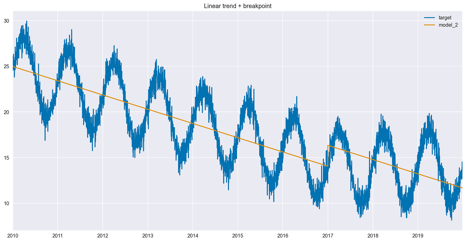
df[["target", "model_2"]].plot(title="Linear trend + breakpoint");
After introducing the breakpoint, there was a vertical jump in the fitted line, but the slope before/after is the same.
Figure 4. Best fit line obtained from a linear model using linear trend and a breakpoint as features

Figure 4 shows a few important changes, as listed below:

  • The fitted line displays a vertical jump, which corresponds to the coefficient by the new Boolean feature.
  • The vertical jump occurs exactly on the first date when the feature becomes active (a value of 1 instead of 0).
  • The slope of the line is the same before and after the introduced breakpoint.
  • The model is trying to compensate for the incorrect slope by adding a fixed amount to the predictions after the breakpoint.

There is no trend in the last 3 years of data, so ideally the line should be close to flat after January 1, 2017. 

Adding an interaction term

To change the slope after the breakpoint, add a more complex dependency on the timestamp (represented by a linear trend). That is exactly what an interaction term does–it is a multiplication of the linear trend and the placeholder variable.

df["interaction_term"] = df["after_2017_breakpoint"] * df["linear_trend"]

X = df[["linear_trend", "after_2017_breakpoint", "interaction_term"]]
y = df[["target"]]

lm = LinearRegression()
lm.fit(X, y)

df["model_3"] = lm.predict(X)

df[["target", "model_3"]].plot(title="Linear trend + breakpoint + interaction term");
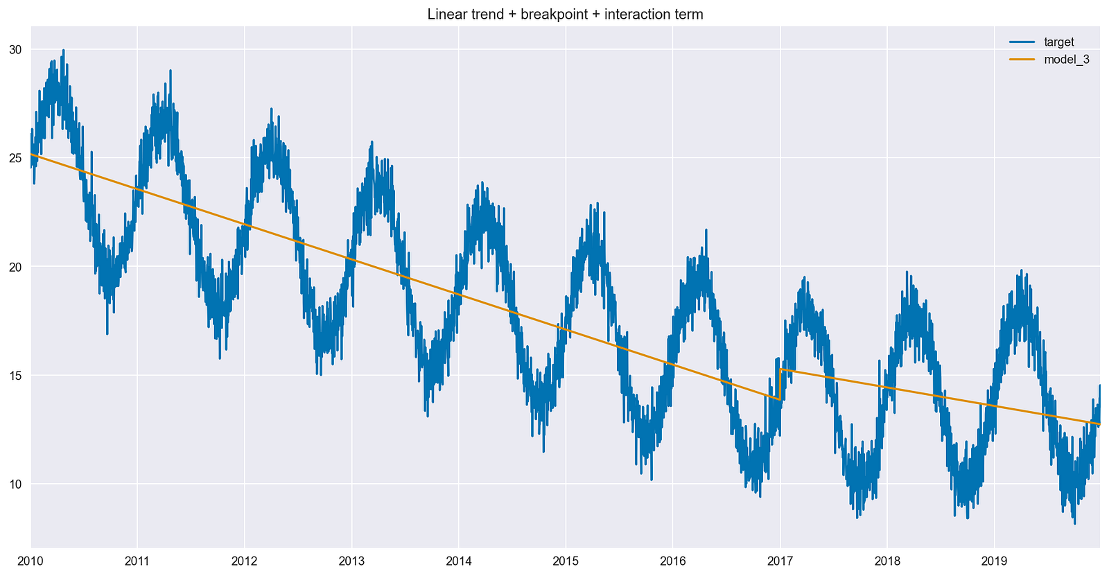
After introducing the interaction term, the slope clearly changes after the breakpoint. It is not as steep anymore.
Figure 5. Best fit line obtained from a linear model using a linear trend, a breakpoint, and an interaction term as features

Figure 5 shows the impact of having the interaction term in the model. Compared to Figure 4, the slope of the best fit line is different after the breakpoint. 

To be more precise, the difference is actually the value of the coefficient by the interaction term. While the new line did not flatten out, it is still less steep than it used to be in the earlier parts of the time series.

Introducing the breakpoint together with an interaction term increased the model’s ability to capture the trend of the time series. In turn, that should increase the predictive performance of the model.

Summary

Using interaction terms can make the specification of a linear model more flexible (different slopes for different lines), which can result in a better fit to the data and better predictive performance. You can add interaction terms as a multiplication of the original features. In the context of time series, you can use interaction terms to better capture any changes to the trend.

Find the code used in this post in A Comprehensive Guide on Interaction Terms in Time Series Forecasting on GitHub. Additionally, the code in the notebook shows how to leverage cuDF and cuML to train your models using GPU acceleration. As always, feedback is welcome. You can reach out to me on Twitter or in the comments.

Categories
Misc

So, So Fresh: Play the Newest Games in the Cloud on Day One

It’s a party this GFN Thursday with several newly launched titles streaming on GeForce NOW. Revel in gaming goodness with Xenonauts 2, Viewfinder and Techtonica, among the four new games joining the cloud this week. Portal fans, stay tuned — the Portal: Prelude RTX mod will be streaming on GeForce NOW to members soon. Plus, Read article >

Categories
Misc

OCI Accelerates HPC, AI, and Database Using RoCE and NVIDIA ConnectX

Oracle is one of the top cloud service providers in the world, supporting over 22,000 customers and reporting revenue of nearly $4 billion per quarter and…
Oracle is one of the top cloud service providers in the world, supporting over 22,000 customers and reporting revenue of nearly $4 billion per quarter and annual growth of greater than 40%. Oracle Cloud Infrastructure (OCI) is growing at an even faster rate and offers a complete cloud infrastructure for every workload. 

Having added 11 regions in the last 18 months, OCI currently offers 41 regions and supports hosted, on-premises, hybrid, and multi-cloud deployments. It enables customers to run a mix of custom-built, third-party ISVs and Oracle applications on a scalable architecture. OCI provides scalable networking and tools to support security, observability, compliance, and cost management. 

One of the differentiators of OCI is its ability to offer high-performance computing (HPC), Oracle Exadata and Autonomous Database, and GPU-powered applications such as AI and machine learning (ML), with fast infrastructure-as-a-service (IaaS) performance that rivals dedicated on-premises infrastructure. A key component to delivering this high performance is a scalable, low-latency network that supports remote direct memory access (RDMA). For more details, see First Principles: Building a High-Performance Network in the Public Cloud.

Networking challenge of HPC and GPU-powered compute 

A commonality across HPC applications, GPU-powered AI workloads, and the Oracle Autonomous Database on Exadata is that they all run as distributed workloads. Data processing occurs simultaneously on multiple nodes, using a few dozen to thousands of CPUs and GPUs. These nodes must communicate with each other, share intermediate results in multi-stage problem solving with gigabytes to petabytes of storage to access common data, and often assemble the results of distributed computing into a cohesive solution. 

These applications require high throughput and low latency to communicate across nodes to solve problems quickly. Amdahl’s law states that the speedup from parallelizing a task is limited by how much of the task is inherently serial and cannot be parallelized. The amount of time needed to transfer information between nodes adds inherently serial time to the task because nodes must wait for the data transfer to complete and for the slowest node in the task to finish before starting the next parallelizable part of the job. 

For this reason, the performance of the cluster network becomes paramount, and an optimized network can enable a distributed compute cluster to deliver results much sooner than the same computing resources running on a slower network. This time-saving speeds job completion and reduces costs. 

What is RDMA? 

RDMA is remote direct memory access, the most efficient means of transferring data between different machines. It enables a server or storage appliance to communicate and share data over a network without making extra copies and without interrupting the host CPU. It is used for AI, big data, and other distributed technical computing workloads. 

Traditional networking interrupts the CPU multiple times and makes multiple copies of the data being transmitted as it passes from the application through the OS kernel, to the adapter, then back up the stack on the receiving end. RDMA uses only one copy of the data on each end and typically bypasses the kernel, placing data directly in the receiving machine’s memory without interrupting the CPU. 

This process enables lower latency and higher throughput on the network and lower CPU utilization for the servers and storage systems. Today, the majority of HPC, technical computing, and AI applications can be accelerated by RDMA. For more details, see How RDMA Became the Fuel for Fast Networks.

What is InfiniBand? 

InfiniBand is a lossless network optimized for HPC, AI, big data, and other distributed technical computing workloads. It typically supports the highest bandwidth available (currently 400 Gbps per connection) for data center networks and RDMA, enabling machines to communicate and share data without interrupting the host CPU. 

InfiniBand adapters offload networking and data movement tasks from the CPU and feature an optimized, efficient networking stack, enabling CPUs, GPUs, and storage to move data rapidly and efficiently. The InfiniBand adapters and switches can also perform specific compute and data aggregation tasks in the network, mostly oriented around message passing interface (MPI) collective operations. 

This in-network computing speeds up distributed applications, enabling faster problem solving. It also frees up server CPU cores and improves energy efficiency. InfiniBand can also automatically balance traffic loads and reroute connections around broken links. 

As a result, many computing clusters that are dedicated to AI, HPC, big data, or other scientific computing run on an InfiniBand network to provide the highest possible performance and efficiency. When distributed computing performance is the top priority, and the adoption of a specialized stack of network adapters, switches, and management is acceptable, InfiniBand is the network of choice. But a data center might choose to run Ethernet instead of InfiniBand, for other reasons.

What is RoCE? 

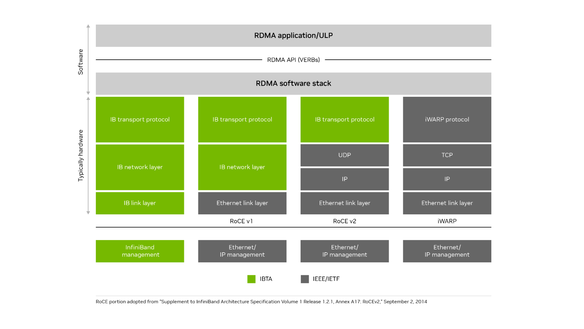
RDMA over Converged Ethernet (RoCE) is an open standard enabling remote direct memory access and network offloads over an Ethernet network. The current and most popular implementation is RoCEv2. It uses an InfiniBand communication layer running on top of UDP (Layer 4) and IP (Layer 3), which runs on top of high-speed Ethernet (Layer 2) connections. 

It also supports remote direct memory access, zero-copy data transfers, and bypassing the CPU when moving data. Using the IP protocol on Ethernet enables RoCEv2 to be routable over standard Ethernet networks. RoCE brings many of the advantages of InfiniBand to Ethernet networks. RoCEv2 runs the InfiniBand transport layer over UDP and IP protocols on an Ethernet network. iWARP ran the iWARP protocol on top of the TCP protocol on an Ethernet network but failed to gain popular adoption because of performance and implementation challenges (Figure 1).

A graphic depicting the OSI transport layer mapped across the RDMA software stack for InfiniBand and Ethernet.
Figure 1. NVIDIA InfiniBand runs the InfiniBand transport layer over an InfiniBand network

How do RoCE networks address scalability?

RoCE operates most efficiently on networks with very low levels of packet loss. Traditionally, small RoCE networks use priority flow control (PFC), based on the IEEE 802.1Qbb specification, to make the network lossless. If any destination is too busy to process all incoming traffic, it sends a pause frame to the next upstream switch port, and that switch holds traffic for the time specified in the pause frame. 

If needed, the switch can also send a pause frame up to the next switch in the fabric and eventually onto the originator of the traffic flow. This flow control avoids having the port buffers overflow on any host or switch and prevents packet loss. You can manage up to eight traffic classes with PFC, each class having its own flows and pauses separate from the others. 

However, PFC has some limitations. It operates only at the Layer 2 (Ethernet) level of the Open System Interconnection (OSI) 7-layer model, so it cannot work across different subnets. While a subnet can have thousands or millions of nodes, a typical subnet is limited to 254 IP addresses and consists of a few racks (often one rack) within a data center, which does not scale for large distributed applications. 

PFC operates on a coarse-grained port level and cannot distinguish between flows sharing that port. Also, if you use PFC in a multi-level switch fabric, congestion at one destination switch for one flow can spread to multiple switches and block unrelated traffic flows that share one port with the congested flow. The solution is usually to implement a form of congestion control.

Congestion management for large RoCE networks

The TCP protocol includes support for congestion management based on dropped packets. When an endpoint or switch is overwhelmed by a traffic flow, it drops some packets. When the sender fails to receive an acknowledgment from the transmitted data, the sender assumes the packet was lost because of network congestion, slows its rate of transmission, and retransmits the presumably lost data. 

This congestion management scheme does not work well for RDMA on Ethernet (and therefore for RoCE). RoCE does not use TCP and  the process of waiting for packets to timeout and then retransmitting the lost data introduces too much latency—and too much variability in latency or jitter—for efficient RoCE operation. 

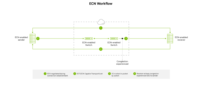
Large RoCE networks often implement a more proactive congestion control mechanism known as explicit congestion notification (ECN), in which the switches mark packets if congestion occurs in the network. The marked packets alert the receiver that congestion is imminent, and the receiver alerts the sender with a congestion notification packet or CNP. After receiving the CNP, the sender knows to back off, slowing down the transmission rate temporarily until the flow path is ready to handle a higher rate of traffic. 

Congestion control works across Layer 3 of the OSI model, so it functions across different subnets and scales up to thousands of nodes. However, it requires setting changes to both switches and adapters supporting RoCE traffic. Implementation details of when switches mark packets for congestion, how quickly senders back off sending data, and how aggressively senders resume high-speed transmissions are all critical to determining the scalability and performance of the RoCE network.

A graphic depicting ECN workflow mapping the progress of experiencing congestion, marketing the packet within the switch, and notifying the sender.
Figure 2. ECN marks outgoing packets as CE–Congestion Experienced when the switch queue is becoming full. The flow recipient receives the packet and notifies the sender to slow transmission

Other Ethernet-based congestion control algorithms include quantized congestion notification (QCN) and data center TCP (DCTCP). In QCN, switches notify flow senders directly with the level of potential congestion, but the mechanism functions only over L2. Consequently, it cannot work across more than one subnet. DCTCP uses the sender’s network interface card (NIC) to measure the round-trip time (RTT) of special packets to estimate how much congestion exists and how much the sender must slow down data transmissions. 

But DCTCP lacks a fast start option to quickly start or resume sending data when no congestion exists, places a heavy load on host CPUs, and does not have a good mechanism for the receiver to communicate with the sender. In any case, DCTCP requires TCP, so it does not work with RoCE. 

Smaller RoCE networks using newer RDMA-capable ConnectX SmartNICs from NVIDIA, or newer NVIDIA BlueField DPUs, can use Zero Touch RoCE (ZTR). ZTR enables excellent RoCE performance without setting up PFC or ECN on the switch, which greatly simplifies network setup. However, initial deployments of ZTR have been limited to small RoCE network clusters, and a more scalable version of ZTR that uses RTT for congestion notification is still in the proving stages. 

How OCI implements a scalable RoCE network 

OCI determined that certain cloud workloads required RDMA for maximum performance. These include AI, HPC, Exadata, autonomous databases, and other GPU-powered applications. Out of the two standardized RDMA options on Ethernet, they chose RoCE for its performance and wider adoption. 

The RoCE implementation needed to scale to run across clusters containing thousands of nodes and deliver consistently low latency to ensure an excellent experience for cloud customers. 

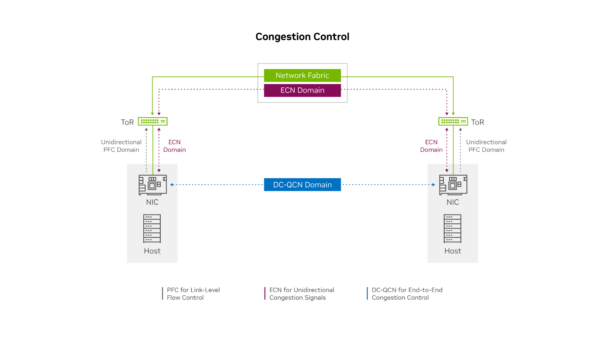
After substantial research, testing, and careful design, OCI decided to customize their own congestion control solution based on the data center quantized congestion notification (DC-QCN) algorithm, which they optimized for different RoCE-accelerated application workloads. The OCI DC-QCN solution is based on ECN with minimal use of PFC.

A graph shows how the OCI network uses RoCE with priority flow control at the link level, explicit congestion notification for unidirectional congestion signaling and data center quantized congestion notification for end-to-end congestion control.
Figure 3. The OCI RoCE network uses ECN across the network fabric plus a limited amount of unidirectional PFC only between the hosts and ToR switches

A separate network for RoCE 

OCI built a separate network for RoCE traffic because the needs of the RDMA network tend to differ from the regular data center network. The different types of application traffic, congestion control, and routing protocols each prefer to have their own queues. Each NIC typically supports only eight traffic classes, and the NIC and switch configuration settings and firmware might be different for RDMA from non-RDMA workloads. For these reasons, having a separate Ethernet network for RoCE traffic and RoCE-accelerated applications makes sense. 

Limited use of PFC at the edge

OCI implemented a limited level of PFC, only unidirectionally at the network edge. Endpoints can ask the top-of-rack (ToR) switch to pause transmission if their NICs buffer fills up. However, the ToR switches never ask the endpoints to pause and do not pass ‌pause requests up the network to leaf or spine switches. This process prevents head-of-line blocking and congestion spreading if the incoming traffic flow rate temporarily exceeds the receiver’s ability to process and buffer data. 

The ECN mechanism ensures that PFC is very rarely needed. In the rare case that a receiving node’s NIC buffer is temporarily overrun while the ECN feedback mechanism is activating, PFC enables the receiving node to briefly pause the incoming data flow until the sender receives the CNPs and slows its transmission rate. 

In this sense, you can use PFC as a last resort safeguard to prevent buffer overrun and packet loss at the network edge (at the endpoints). OCI envisions that with the next generation of ConnectX SmartNICs, you might not need PFC, even at the edge of the network. 

Multiple classes of congestion control 

OCI determined that they need at least three customized congestion control profiles within DC-QCN for different workloads. Even within the world of distributed applications that require RDMA networking, the needs vary across the following categories:

  • Latency sensitive, requiring consistently low latency throughput
  • Sensitive, high throughput
  • Mixed, requires a balance of low-latency and high throughput

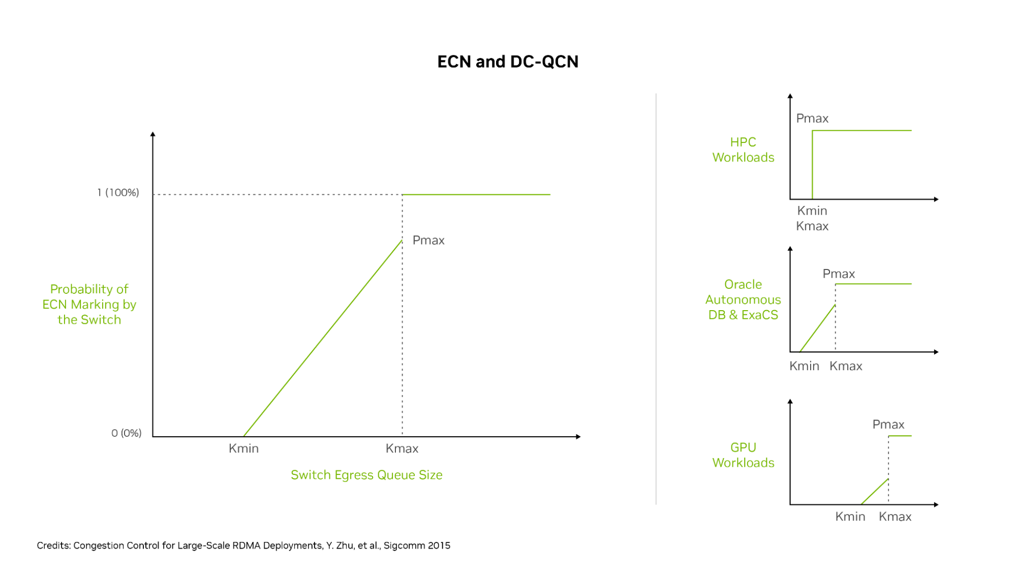
The primary setting for customizing congestion control is the probability P (ranging from 0 to 1) of the switch adding the ECN marking to an outgoing packet, based on queue thresholds Kmin and Kmax. P starts at 0 when the switch queue is not busy, which means it has no chance of congestion. 

When the port queue reaches Kmin, the value P rises above 0, increasing the chance that any packet is marked with ECN. When the queue fills to value Kmax, P is set to Pmax (typically 1), meaning every outgoing packet of that flow on that switch is marked with ECN. Different DC-QCN profiles typically have a no-congestion range where P is 0, a potential congestion range where P is between 0 and 1, and a congestion range where P is 1. 

A more aggressive set of thresholds has lower values for Pmin and Pmax, resulting in earlier ECN packet marking and lower latency but possibly also lower maximum throughput. A relaxed set of thresholds has higher values for Pmin and Pmax, marking fewer packets with ECN, resulting in some higher latencies but also higher throughput. 

To the right side of Figure 4 are three examples of OCI workloads: HPC, Oracle Autonomous DataBase and Exadata Cloud Service, and GPU workloads. These services use different RoCE congestion control profiles. HPC workloads are latency-sensitive and give up some throughput to guarantee lower latency. ‌Consequently, Kmin and Kmax are identical and low (aggressive), and at a low amount of queuing, they mark 100% of all packets with ECN. 

Most GPU workloads are more forgiving on latency but need maximum throughput. The DC-QCN profile gradually marks more packets as buffers ramp from Kmin to Kmax and sets those values relatively higher to enable switch buffers to get closer to full before signaling to flow endpoints that they slow down. 

For Autonomous Database and Exadata Cloud Service workloads, the required balance of latency and bandwidth is in between. Marking or increasing P value gradually increases between Kmin and Kmax, but these values are set at lower threshold values than for GPU workloads.  

A graphic showing four line graphs comparing how optimal network congestion control is achieved by varying data center quantized congestion notification thresholds on different services.
Figure 4. OCI sets DC-QCN to use different Kmin and Kmax thresholds for ECN packet marking, resulting in optimized network behavior on their RoCE network for different workloads

With these settings, HPC flows get 100% ECN packet marking as soon as the queues hit the Kmin level (which is the same here as Kmax) for early and aggressive congestion control engagement. Oracle Autonomous Database and Exadata flows see moderately early ECN marking, but only a portion of packets is marked until buffers reach the Kmax level. 

Other GPU workloads have a higher Kmin setting so ECN marking does not begin until switch queues are relatively fuller, and 100% ECN marking only happens when the queues are close to full. Different workloads get the customized congestion control settings needed to provide the ideal balance of latency and throughput for maximum application performance. 

Leveraging advanced network hardware

An important factor in achieving high performance for RoCE networks is the type of network card used. The NIC offloads the networking stack, including RDMA, to a specialized chip to offload the work from the CPUs and GPUs. OCI uses ConnectX SmartNICs, which have market-leading network performance for both TCP and RoCE traffic. 

These SmartNICs also support rapid PFC and ECN reaction times for detecting ECN-marked packets or PFC pause frames, sending CNPs, and adjusting the data transmission rates downward and upward in response to congestion notifications. 

NVIDIA has been a long time leader in the development and support of RDMA, PFC, ECN, and DC-QCN technology, and a leader in high-performance GPUs and GPU connectivity. The advanced RoCE offloads in ConnectX enable higher throughput and lower latency on the OCI network, and their rapid, hardware-based ECN reaction times help ensure that DC-QCN functions smoothly.

By implementing an optimized congestion control scheme on a dedicated RoCE network, plus a combination of localized PFC, multiple congestion control profiles, and NVIDIA network adapters, OCI has built a very scalable cluster network. It’s ideal for distributed workloads, such as AI and ML, HPC, and Oracle Autonomous Database, and delivers high throughput and low-latency performance close to what an InfiniBand network can achieve.  

Emphasizing data locality

With optimizing cluster network performance, OCI also manages data locality to minimize latency. With the large size of RoCE-connected clusters that often span multiple data center racks and halls, even in an era of 100-, 200-, and 400-Gbps networking connections, the speed of light has not changed, and longer cables result in higher latency. 

Connections to different halls in the data center traverse more switches, and each switch hop adds some nanoseconds to connection latency. OCI shares server locality information with both its customers and the job scheduler, so they can schedule jobs to use servers and GPUs that are close to each other in the network. 

For example, the NVIDIA Collective Communication Library (NCCL) understands the OCI network topology and server locality information and can schedule GPU work accordingly. So, the compute and storage connections traverse fewer switch hops and shorter cable lengths, to reduce the average latency within the cluster. 

It also sends less traffic to spine switches, simplifying traffic routing and load-balancing decisions. OCI also worked with its switch vendors to make the switches more load-aware, so flows can be routed to less-busy connections. Each switch generally has two connections up and down the network, enabling multiple datapaths for any flow. 

Conclusion

By investing in a dedicated RoCE network with an optimized implementation of DC-QCN, advanced ConnectX NICs, and customized congestion control profiles, OCI delivers a highly scalable cluster that supports accelerated computing for many different workloads and applications. OCI cluster networks simultaneously deliver high throughput and low latency. For small clusters, latency-half the round trip time-can be as little as 2 microseconds. For large clusters, latency is typically under 4 microseconds. For extremely large superclusters, latencies are in the range of 4-8 microseconds, with most traffic seeing latencies at the lower end of this range. 

Oracle Cluster Infrastructure uses an innovative approach to deliver scalable, RDMA-powered networking on Ethernet for a multitude of distributed workloads, providing higher performance and value to their customers. 

For more information, see the following resources:

Categories
Misc

Programming the Quantum-Classical Supercomputer

Heterogeneous computing architectures—those that incorporate a variety of processor types working in tandem—have proven extremely valuable in the continued…
Heterogeneous computing architectures—those that incorporate a variety of processor types working in tandem—have proven extremely valuable in the continued scalability of computational workloads in AI, machine learning (ML), quantum physics, and general data science. 

Critical to this development has been the ability to abstract away the heterogeneous architecture and promote a framework that makes designing and implementing such applications more efficient. The most well-known programming model that accomplishes this is CUDA Toolkit, which enables offloading work to thousands of GPU cores in parallel following a single-instruction, multiple-data model. 

Recently, a new form of node-level coprocessor technology has been attracting the attention of the computational science community: the quantum computer, which relies on the non-intuitive laws of quantum physics to process information using principles such as superposition, entanglement, and interference. This unique accelerator technology may prove useful in very specific applications and is poised to work in tandem with CPUs and GPUs, ushering in an era of computational advances previously deemed unfeasible. 

The question then becomes: If you enhance an existing classically heterogeneous compute architecture with quantum coprocessors, how would you program it in a manner fit for computational scalability?

NVIDIA is answering this question with CUDA Quantum, an open-source programming model extending both C++ and Python with quantum kernels intended for compilation and execution on quantum hardware. 

This post introduces CUDA Quantum, highlights its unique features, and demonstrates how researchers can leverage it to gather momentum in day-to-day quantum algorithmic research and development. 

CUDA Quantum: Hello quantum world 

To begin with a look at the CUDA Quantum programming model, create a two-qubit GHZ state with the Pythonic interface. This will accustom you to its syntax.

import cudaq

# Create the CUDA Quantum Kernel
kernel = cudaq.make_kernel()

# Allocate 2 qubits
qubits = kernel.qalloc(2)

# Prepare the bell state
kernel.h(qubits[0]) 
kernel.cx(qubits[0], qubits[1])

# Sample the final state generated by the kernel 
result = cudaq.sample(kernel, shots_count = 1000) 

print(result) 

{11:487, 00:513}

The language specification borrows concepts that CUDA has proven successful; specifically, the separation of host and device code at the function boundary level. The code snippet below demonstrates this functionality on a GHZ state preparation example in C++. 

#include 

int main() {
      // Define the CUDA Quantum kernel as a C++ lambda
	auto ghz =[](int numQubits) __qpu__ {
           // Allocate a vector of qubits
		cudaq::qvector q(numQubits);

           // Prepare the GHZ state, leverage standard 
           // control flow, specify the x operation 
           // is controlled. 
		h(q[0]);
		for (int i = 0; i (q[i], q[i + 1]);
	};

     // Sample the final state generated by the kernel
auto results = cudaq::sample(ghz, 15); 
results.dump();

return 0;
}

CUDA Quantum enables the definition of quantum code as stand-alone kernel expressions. These expressions can be any callable in C++ (a lambda is shown here, and implicitly typed callable) but must be annotated with the __qpu__ attribute enabling the nvq++ compiler to compile them separately. Kernel expressions can take classical input by value (here the number of qubits) and leverage standard C++ control flow, for example for loops and if statements. 

The utility of GPUs

The experimental efforts to scale up QPUs and move them out of research labs and host them on the cloud for general access have been phenomenal. However, current QPUs are noisy and small-scale, hindering advancement of algorithmic research. To aid this, circuit simulation techniques are answering the pressing requirements to advance research frontiers. 

Desktop CPUs can simulate small-scale qubit statistics; however, memory requirements of the state vector grow exponentially with the number of qubits. A typical desktop computer possesses eight GB of RAM, enabling one to sluggishly simulate approximately 15 qubits. The  latest NVIDIA DGX H100 enables you to surpass the 35-qubit mark with unparalleled speed. 

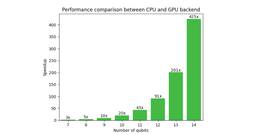
Figure 1 shows a comparison of CUDA Quantum on CPU and GPU backend for a typical variational algorithmic workflow. The need for GPUs is evident here, as the speedup at 14 qubits is 425x and increases with qubit count. Extrapolating to 30 qubits, the CPU-to-GPU runtime is 13 years, compared to 2 days. This unlocks researchers’ abilities to go beyond small-scale proof of concept results to implementing algorithms closer to real-world applications.

Bar graph showing performance improvements in execution time between a CPU and GPU as a function of number of qubits. At 14 qubits, the GPU is 425 times faster than the CPU.
Figure 1. Performance comparison between CPU and GPU for a typical quantum neural network workflow as a function of qubit count 

Along with CUDA Quantum, NVIDA has developed cuQuantum, a library enabling lightning-fast simulation of a quantum computer using both state vector and tensor network methods through hand-optimized CUDA kernels. Memory allocation and processing happens entirely on GPUs resulting in dramatic increases in performance and scale. CUDA Quantum in combination with cuQuantum forms a powerful platform for hybrid algorithm research. 

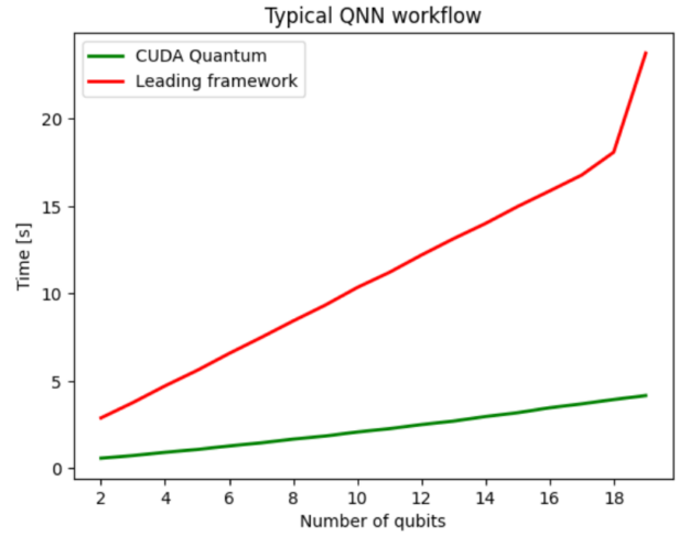
Figure 2 compares CUDA Quantum with a leading quantum computing SDK, both leveraging the NVIDIA cuQuantum backend to optimally offload circuit simulation onto NVIDIA GPUs. In this case, the benefits of using CUDA Quantum are isolated and yield a 5x performance improvement on average compared to a leading framework. 

 Line plot showing the execution time for a typical quantum neural network workflow as a function of number of qubits for CUDA Quantum and a leading framework. CUDA Quantum is on average 5x faster. Since both frameworks were executed on GPUs, we are isolating the performance benefits of using CUDA Quantum.
Figure 2. GPU-to-GPU comparison between CUDA Quantum and a leading framework, both offloading circuit simulation to NVIDIA GPUs, with CUDA Quantum on average 5x faster

Enabling multi-QPU workflows of the future

CUDA Quantum is not limited to consideration of current cloud-based quantum execution models, but is fully anticipating tightly coupled, system-level quantum acceleration. Moreover, CUDA Quantum enables application developers to envision workflows for multi-QPU architectures with multi-GPU backends. 

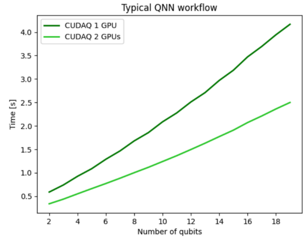
For the preceding quantum neural network (QNN) example, you can use the multi-GPU functionality to run a forward pass of the dataset enabling us to perform multi-QPU workflows of the future. Figure 3 shows results for distributing the QNN workflow across two GPUs and demonstrates strong scaling performance indicating effective usage of all GPU compute resources. Using two GPUs makes the overall workflow twice as fast compared to a single GPU, demonstrating strong scaling. 

Line plot showing the execution time of a typical quantum neural network workflow as a function of the number of qubits. The execution time is approximately half when two GPUs are used in comparison to a single GPU.
Figure 3. ‌Results for distributing the QNN forward pass workload to multiple QPUs enabled ‌by the multi-GPU backend

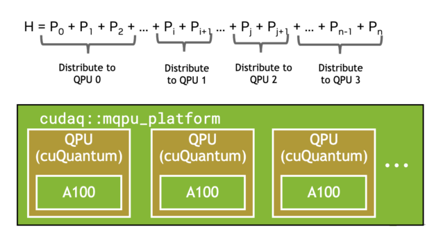
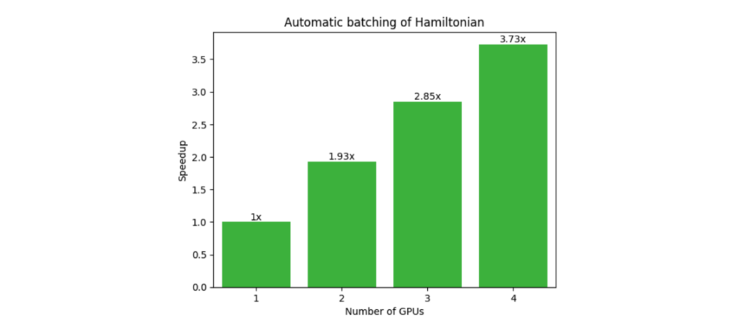
Another common workflow that benefits from multi-QPU parallelization is the Variational Quantum Eigensolver (VQE). This requires the expectation value of a composite Hamiltonian made up of multiple single Pauli tensor product terms. The CUDA Quantum observe call, shown below, automatically batches terms (Figure 4), and offloads to multiple GPUs or QPUs if available, demonstrating strong scaling (Figure 5). 

numQubits, numTerms = 30, 1e5
hamiltonian = cudaq.SpinOperator.random(numQubits, numTerms)
cudaq.observe(ansatz, hamiltonian, parameters)
Image showing a Hamiltonian composed of many terms being batched into four groups and offloaded to four GPUs.
Figure 4. Automatic batching of Hamiltonian terms across multiple NVIDIA A100 GPUs
Bar graph showing speedup in execution time gained by automatically batching a Hamiltonian composed of multiple terms into four batches and executing on four GPUs. The speedups gained demonstrate strong scaling.
Figure 5. Speedups gained due to an optimized software stack supporting the hardware available to the user, GPUs or QPUs

GPU-QPU workflows 

This post has so far explored using GPUs for scaling quantum circuit simulation beyond what is possible on CPUs, as well as multi-QPU workflows. The following sections dive into true heterogeneous computing with a hybrid quantum neural network example using PyTorch and CUDA Quantum.

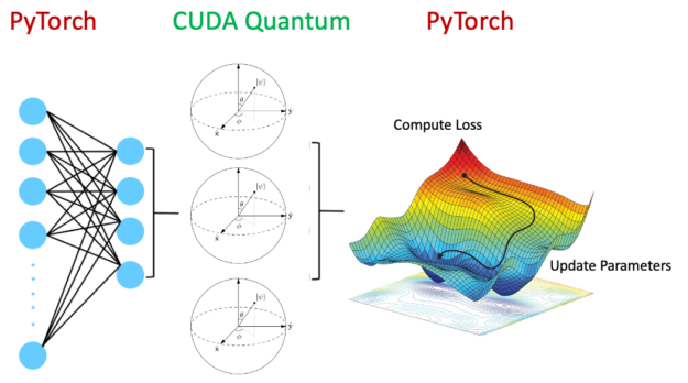
As shown in Figure 6, a hybrid quantum neural network encompasses a quantum circuit as a layer within the overall neural network architecture. An active area of research, this is poised to be advantageous in certain areas, improving generalization errors.

Image showing layers of neural network nodes, the output of which acts as the input to a quantum circuit, which is measured to generate the loss function. This workflow enables one to integrate PyTorch layers with CUDA Quantum.
Figure 6. Hybrid quantum neural network architecture accelerated by GPUs made possible by CUDA Quantum

Evidently, it is advantageous to run the classical neural network layers on GPUs and the quantum circuits on QPUs. Accelerating the whole workflow with CUDA Quantum is made possible by setting the following: 

quantum_device = cudaq.set_target('ion-trap')
classical_device = torch.cuda.set_device(gpu0)

The utility of this is profound. CUDA Quantum enables offloading relevant kernels suited for QPUs and GPUs in a tightly integrated, seamless fashion. In addition to hybrid applications, workflows involving error correction, real-time optimal control, and error mitigation through Clifford data regression would all benefit from tightly coupled compute architectures. 

QPU hardware providers 

The foundational information unit embedded within the CUDA Quantum programming paradigm is the qudit, which represents a quantum bit capable of accessing d-states. Qubit is a specific instance where d=2. By using qudits, CUDA Quantum can efficiently target diverse quantum computing architectures, including superconducting circuits, ion traps, neutral atoms, diamond-based, photonic systems, and more. 

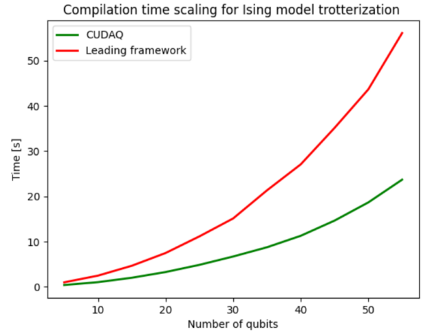
You can conveniently develop workflows, and the nvq++ compiler automatically compiles and executes the program on the designated architecture. Figure 7 shows the compilation speedups that the novel compiler yields. Compilation involves circuit optimization, decomposing into the native gate sets supported by the hardware and qubit routing. The nvq++ compiler used by CUDA Quantum is on average 2.4x faster compared to its competition.

Line graph showing how the compilation time scales with number of qubits for CUDA Quantum and a leading framework. The novel ‌compiler used by CUDA Quantum is on average 2.4x faster and its rate of increase (gradient) is also much shallower in comparison.
Figure 7. Compilation time scaling with the number of qubits for CUDA Quantum and a leading framework

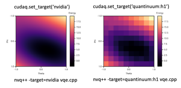
To accommodate the desired backend, you can simply modify the set_target() flag. Figure 8 shows an example of how you can seamlessly switch between the simulated backend and the Quantinuum H1 ion trap system. The top shows the syntax to set the desired backend in Python and the bottom in C++. 

Image showing a heatmap of the cost landscape generated by a VQE workflow being executed on cuQuantum simulated backed and the Quantinuum H1 processor. The ease with which users can change the backend and the syntax enabling this in Python and C++ is highlighted.
Figure 8. VQE landscape plots demonstrating execution on simulated or QPU hardware

Getting started with CUDA Quantum

This post has just briefly touched on some of the features of the CUDA Quantum programming model. Reach out to the CUDA Quantum community on GitHub and get started with some example code snippets. We are excited to see the research CUDA Quantum enables for you. 

Categories
Misc

Sailing Seas of Data: Startup Charts Autonomous Oceanic Monitoring

Saildrone is making a splash in autonomous oceanic monitoring. The startup’s nautical data collection technology has tracked hurricanes up close in the North Atlantic, discovered a 3,200-foot underwater mountain in the Pacific Ocean and begun to help map the entirety of the world’s ocean floor. Based in the San Francisco Bay Area, the company develops Read article >

Categories
Offsites

SimPer: Simple self-supervised learning of periodic targets

Learning from periodic data (signals that repeat, such as a heart beat or the daily temperature changes on Earth’s surface) is crucial for many real-world applications, from monitoring weather systems to detecting vital signs. For example, in the environmental remote sensing domain, periodic learning is often needed to enable nowcasting of environmental changes, such as precipitation patterns or land surface temperature. In the health domain, learning from video measurement has shown to extract (quasi-)periodic vital signs such as atrial fibrillation and sleep apnea episodes.

Approaches like RepNet highlight the importance of these types of tasks, and present a solution that recognizes repetitive activities within a single video. However, these are supervised approaches that require a significant amount of data to capture repetitive activities, all labeled to indicate the number of times an action was repeated. Labeling such data is often challenging and resource-intensive, requiring researchers to manually capture gold-standard temporal measurements that are synchronized with the modality of interest (e.g., video or satellite imagery).

Alternatively, self-supervised learning (SSL) methods (e.g., SimCLR and MoCo v2), which leverage a large amount of unlabeled data to learn representations that capture periodic or quasi-periodic temporal dynamics, have demonstrated success in solving classification tasks. However, they overlook the intrinsic periodicity (i.e., the ability to identify if a frame is part of a periodic process) in data and fail to learn robust representations that capture periodic or frequency attributes. This is because periodic learning exhibits characteristics that are distinct from prevailing learning tasks.

Feature similarity is different in the context of periodic representations as compared to static features (e.g., images). For example, videos that are offset by short time delays or are reversed should be similar to the original sample, whereas videos that have been upsampled or downsampled by a factor x should be different from the original sample by a factor of x.

To address these challenges, in “SimPer: Simple Self-Supervised Learning of Periodic Targets”, published at the eleventh International Conference on Learning Representations (ICLR 2023), we introduced a self-supervised contrastive framework for learning periodic information in data. Specifically, SimPer leverages the temporal properties of periodic targets using temporal self-contrastive learning, where positive and negative samples are obtained through periodicity-invariant and periodicity-variant augmentations from the same input instance. We propose periodic feature similarity that explicitly defines how to measure similarity in the context of periodic learning. Moreover, we design a generalized contrastive loss that extends the classic InfoNCE loss to a soft regression variant that enables contrasting over continuous labels (frequency). Next, we demonstrate that SimPer effectively learns period feature representations compared to state-of-the-art SSL methods, highlighting its intriguing properties including better data efficiency, robustness to spurious correlations, and generalization to distribution shifts. Finally, we are excited to release the SimPer code repo with the research community.

The SimPer framework

SimPer introduces a temporal self-contrastive learning framework. Positive and negative samples are obtained through periodicity-invariant and periodicity-variant augmentations from the same input instance. For temporal video examples, periodicity-invariant changes are cropping, rotation or flipping, whereas periodicity-variant changes involve increasing or decreasing the speed of a video.

To explicitly define how to measure similarity in the context of periodic learning, SimPer proposes periodic feature similarity. This construction allows us to formulate training as a contrastive learning task. A model can be trained with data without any labels and then fine-tuned if necessary to map the learned features to specific frequency values.

Given an input sequence x, we know there’s an underlying associated periodic signal. We then transform x to create a series of speed or frequency altered samples, which changes the underlying periodic target, thus creating different negative views. Although the original frequency is unknown, we effectively devise pseudo- speed or frequency labels for the unlabeled input x.

Conventional similarity measures such as cosine similarity emphasize strict proximity between two feature vectors, and are sensitive to index shifted features (which represent different time stamps), reversed features, and features with changed frequencies. In contrast, periodic feature similarity should be high for samples with small temporal shifts and or reversed indexes, while capturing a continuous similarity change when the feature frequency varies. This can be achieved via a similarity metric in the frequency domain, such as the distance between two Fourier transforms.

To harness the intrinsic continuity of augmented samples in the frequency domain, SimPer designs a generalized contrastive loss that extends the classic InfoNCE loss to a soft regression variant that enables contrasting over continuous labels (frequency). This makes it suitable for regression tasks, where the goal is to recover a continuous signal, such as a heart beat.

SimPer constructs negative views of data through transformations in the frequency domain. The input sequence x has an underlying associated periodic signal. SimPer transforms x to create a series of speed or frequency altered samples, which changes the underlying periodic target, thus creating different negative views. Although the original frequency is unknown, we effectively devise pseudo speed or frequency labels for unlabeled input x (periodicity-variant augmentations τ). SimPer takes transformations that do not change the identity of the input and defines these as periodicity-invariant augmentations σ, thus creating different positive views of the sample. Then, it sends these augmented views to the encoder f, which extracts corresponding features.

Results

To evaluate SimPer’s performance, we benchmarked it against state-of-the-art SSL schemes (e.g., SimCLR, MoCo v2, BYOL, CVRL) on a set of six diverse periodic learning datasets for common real-world tasks in human behavior analysis, environmental remote sensing, and healthcare. Specifically, below we present results on heart rate measurement and exercise repetition counting from video. The results show that SimPer outperforms the state-of-the-art SSL schemes across all six datasets, highlighting its superior performance in terms of data efficiency, robustness to spurious correlations, and generalization to unseen targets.

Here we show quantitative results on two representative datasets using SimPer pre-trained using various SSL methods and fine-tuned on the labeled data. First, we pre-train SimPer using the Univ. Bourgogne Franche-Comté Remote PhotoPlethysmoGraphy (UBFC) dataset, a human photoplethysmography and heart rate prediction dataset, and compare its performance to state-of-the-art SSL methods. We observe that SimPer outperforms SimCLR, MoCo v2, BYOL, and CVRL methods. The results on the human action counting dataset, Countix, further confirm the benefits of SimPer over others methods as it notably outperforms the supervised baseline. For the feature evaluation results and performance on other datasets, please refer to the paper.

Results of SimCLR, MoCo v2, BYOL, CVRL and SimPer on the Univ. Bourgogne Franche-Comté Remote PhotoPlethysmoGraphy (UBFC) and Countix datasets. Heart rate and repetition count performance is reported as mean absolute error (MAE).

Conclusion and applications

We present SimPer, a self-supervised contrastive framework for learning periodic information in data. We demonstrate that by combining a temporal self-contrastive learning framework, periodicity-invariant and periodicity-variant augmentations, and continuous periodic feature similarity, SimPer provides an intuitive and flexible approach for learning strong feature representations for periodic signals. Moreover, SimPer can be applied to various fields, ranging from environmental remote sensing to healthcare.

Acknowledgements

We would like to thank Yuzhe Yang, Xin Liu, Ming-Zher Poh, Jiang Wu, Silviu Borac, and Dina Katabi for their contributions to this work.

Categories
Misc

Advanced API Performance: Pipeline State Objects

A graphic of a computer sending code to multiple stacks.Pipeline state objects (PSOs) define how input data is interpreted and rendered by the hardware when submitting work to the GPUs. Proper management of PSOs is…A graphic of a computer sending code to multiple stacks.

Pipeline state objects (PSOs) define how input data is interpreted and rendered by the hardware when submitting work to the GPUs. Proper management of PSOs is essential for optimal usage of system resources and smooth gameplay.

Recommended:

  • Create PSOs on worker threads asynchronously.
    • PSO creation is where shaders compilation and related stalls happen.
  • Start with generic PSOs with generic shaders that compile quickly and generate specializations later.
    • This gets you up and running faster even if you are not running the most optimal PSO or shader yet.
    • Shaders shared between PSOs will only compile once.
  • Avoid runtime PSO compilations as they most likely will lead to stalls.
    • The driver-managed shader disk cache may come to the rescue.
  • Use PSO libraries.
  • Use identical sensible defaults for don’t care fields wherever possible.
    • This allows for more possibilities for PSO reuse
  • Use the /all_resources_bound / D3DCOMPILE_ALL_RESOURCES_BOUND compile flag if possible.
    • The compiler can do a better job at optimizing texture accesses. 
  • Arrange draw calls by PSO & tessellation usage.
  • Remember that PSO creation is where shaders are compiled and stalls are introduced.
    • It is really important to create PSO asynchronously and early enough before they are used.
    • Tread carefully with thread priorities for PSO compilation threads.
    • Use Idle priority if there is no ‘hurry’ to prevent slowdowns for game threads.
    • Consider temporarily boosting priorities when there is a ‘hurry’

Not recommended:

  • Toggling between compute and graphics on the same command queue more than necessary.
    • This is still a heavyweight switch to make.
  • Toggling tessellation on/off more than necessary.
    • This is also a heavyweight switch to make.
    • It is really important to create PSO asynchronously and early enough before they are used.
    • Tread carefully with thread priorities for PSO compilation threads.
    • Use Idle priority if there is no ‘hurry’ to prevent slowdowns for game threads.
    • Consider temporarily boosting priorities when there is a ‘hurry’
  • Using FXC to generate DXBC in DX12.
    • This causes extra DXBC to DXIL translation, increasing compilation time and PSO library size.
  • Serializing very large (hundreds of thousands) numbers of PSOs to disk in PSO libraries at once.
    • This may significantly bloat the usage of system memory.
    • Use the “miss and update the PSO library” strategy instead.

This post covers best practices when working with pipeline state objects on NVIDIA GPUs. To get a high and consistent frame rate in your applications, see all Advanced API Performance tips.

Acknowledgments

Thanks to Patrick Neil and Dhiraj Kumar for their advice and assistance.

Categories
Misc

Developing a Pallet Detection Model Using OpenUSD and Synthetic Data

Stacked palletsImagine you are a robotics or machine learning (ML) engineer tasked with developing a model to detect pallets so that a forklift can manipulate them. ‌You are…Stacked pallets

Imagine you are a robotics or machine learning (ML) engineer tasked with developing a model to detect pallets so that a forklift can manipulate them. ‌You are familiar with traditional deep learning pipelines, you have curated manually annotated datasets, and you have trained successful models. 

You are ready for the next challenge, which comes in the form of large piles of densely stacked pallets. You might wonder, where should I begin? ‌Is 2D bounding box detection or instance segmentation most useful for this task? ‌Should I do 3D bounding box detection and, if so, how will I annotate it? ‌Would it be best to use a monocular camera, stereo camera, or lidar for detection? ‌Given the sheer quantity of pallets that occur in natural warehouse scenes, manual annotation will not be an easy endeavor. And if I get it wrong, it could be costly.

This is what I wondered when faced with a similar situation. Fortunately, I had an easy way to get started with relatively low commitment: synthetic data.

Overview of synthetic data

Synthetic Data Generation (SDG) is a technique for generating data to train neural networks using rendered images rather than real-world images. ‌The advantage of using synthetically rendered data is that you implicitly know the full shape and location of objects in the scene and can generate annotations like 2D bounding boxes, keypoints, 3D bounding boxes, segmentation masks, and more. ‌

Synthetic data can be a great way to bootstrap a deep learning project, as it enables you to rapidly iterate on ideas before committing to large manual data annotation efforts or in cases where data is limited, restricted, or simply does not exist. For such cases, you might find that synthetic data with domain randomization works very well for your application out-of-the-box first try. ‌And viola–you save time. 

Alternatively, you might find that you need to redefine the task or use a different sensor modality.  Using synthetic data, you can experiment with these decisions without committing to a costly annotation effort.  

In many cases, you may still benefit from using some real-world data. ‌The nice part is, by experimenting with synthetic data you will have more familiarity with the problem, and can invest your annotation effort where it counts the most. Each ML task presents its own challenges, so it is difficult to determine exactly how synthetic data will fit in, whether you will need to use real-world data, or a mix of synthetic and real data.  

Using synthetic data to train a pallet segmentation model

When considering how to use synthetic data to train a pallet detection model, our team started small. Before we considered 3D box detection or anything complex, we first wanted to see if we could detect anything at all using a model trained with synthetic data. To do so, we rendered a simple dataset of scenes containing just one or two pallets with a box on top. ‌We used this data to train a semantic segmentation model.  

We chose to train a semantic segmentation model because the task is well defined and the model architectures are relatively simple. It is also possible to visually identify where the model is failing (the incorrectly segmented pixels).

To train the segmentation model, the team first rendered coarse synthetic scenes (Figure 1).

A rendering of two pallets with a box on top. ‌The rendering is coarse, and the box is a uniform gray color.
Figure 1. A coarse synthetic rendering of two pallets with a box on top

The team suspected that these rendered images alone would lack the diversity to train a meaningful pallet detection model. ‌We also decided to experiment with augmenting the synthetic renderings using generative AI to produce more realistic images.‌ Before training, we applied generative AI to these images to add variation that we believed would improve the ability of the model to generalize to the real world.  

This was done using a depth conditioned generative model, which roughly preserved the pose of objects in the rendered scene. Note that using generative AI is not required when working with SDG. You could also try using traditional domain randomization, like varying the synthetic textures, colors, location, and orientation of the pallets. ‌You may find that traditional domain randomization by varying the rendered textures is sufficient for the application.

An image of the synthetically rendered scene augmented using generative AI.  The augmented image looks photorealistic, and the uniform gray box is replaced with a plastic wrapped box.
Figure 2. The synthetic rendering, augmented using generative AI

After rendering about 2,000 of these synthetic images, we trained a resnet18-based Unet segmentation model using PyTorch. ‌Quickly, the results showed great promise on real-world images (Figure 3).

An image showing a single pallet with a box on top. ‌The pallet is highlighted in green to show the semantic segmentation result.
Figure 3. Real-world pallet image, tested with segmentation model 

The model could accurately segment the pallet. Based on this result, we developed more confidence in the workflow, but the challenge was far from over. Up to this point, the team’s approach did not distinguish between instances of pallets, and it did not detect pallets that were not placed on the floor. ‌For images like the one shown in Figure 4, the results were barely usable. This likely meant that we needed to adjust our training distribution.

An image showing the semantic segmentation results on a warehouse scene with pallets and stacked boxes.  The segmentation model fails to detect pallets that aren't on the floor.
Figure 4. Semantic segmentation model fails to detect stacked pallets

Iteratively increasing the data diversity to improve accuracy

To improve the accuracy of the segmentation model, the team added more images of a wider variety of pallets stacked in different random configurations. We added about 2,000 more images to our dataset, bringing the total to about 4,000 images. ‌We created the stacked pallet scenes using the USD Scene Construction Utilities open-source project. 

USD Scene Construction Utilities was used to position pallets relative to each other in configurations that reflect the distribution you might see in the real world. ‌We used Universal Scene Description (OpenUSD) SimReady Assets, which offered a large diversity of pallet models to choose from.

Images of stacked pallets rendered using Omniverse Replicator.  The pallets vary in type, color and orientation.
Figure 5. Structured scenes created using the USD Python API and USD Scene Construction Utilities, and further randomized and rendered with Omniverse Replicator

Training with the stacked pallets, and with a wider variety of viewpoints, we were able to improve the accuracy of the model for these cases.

If adding this data helped the model, why generate only 2,000 images if there is no added annotation cost? We did not start with many images because we were sampling from the same synthetic distribution. ‌Adding more images would not necessarily add much diversity to our dataset. Instead, we might just be adding many similar images without‌ improving the model’s real-world accuracy.  

Starting small enabled the team to quickly train the model, see where it failed, and adjust the SDG pipeline and add more data. ‌For example, after noticing the model had a bias towards specific colors and shapes of pallets, we added more synthetic data to address these failure cases.

A rendering of scenes containing plastic pallets in many different colors.
Figure 6. ‌A rendering of plastic pallets in various colors

These data variations improved the model’s ability to handle the failure scenarios it encountered (plastic and colored pallets).

If data variation is good, why not just go all-out and add a lot of variation at once? Until our team began testing on real-world data, it was difficult to tell what variance might be required. ‌We might have missed important factors needed to make the model work well. Or, we might have overestimated the importance of other factors, exhausting our effort unnecessarily. ‌By iterating, we better understood what data was needed for the task.

Extending the model for pallet side face center detection

Once we had some promising results with segmentation, the next step was to adjust the task from semantic segmentation to something more practical. ‌We decided that the simplest next task to evaluate was detecting the center of the pallet side faces. 

An image showing a rendered sample with a heat map overlaid on top of the center of the pallet’s side faces.
Figure 7. Example data for the pallet side face center detection task

The pallet side face center points are where a forklift would center itself when manipulating the pallet. ‌While more information may be necessary in practice to manipulate the pallet (such as the distance and angle at this point), we considered this point a simple next step in this process that enables the team to assess how useful our data is for any downstream application.  

Detecting these points could be done with heat map regression, which, like segmentation, is done in the image domain, is easy to implement, and simple to visually interpret. ‌By training a model for this task, we could quickly assess how useful our synthetic dataset is at training a model to detect important key points for manipulation.

The results after training were promising, as shown in Figure 8.

Multiple images showing the heat maps of the pallet side face detection model in multiple scenarios. ‌The scenarios include pallets side by side on the floor, pallets stacked neatly on top of each other, and pallets stacked with boxes.
Figure 8. Real-world detection results for the pallet side face detection model

The team confirmed the ability to detect the pallet side faces using synthetic data, even with closely stacked pallets. We continued to iterate on the data, model, and training pipeline to improve the model for this task. 

Extending the model for corner detection

‌When we reached a satisfactory point for the side face center detection model, we explored taking the task to the next level: detecting the corners of the box.  The initial approach was to use a heat map for each corner, similar to the approach for the pallet side face centers.

An image showing the heatmap detection for the corners of a pallet with a box on top.  The heat map for the corners that are occluded are blurry, indicating the difficulty the model has in predicting the precise location of these points.
Figure 9. ‌Pallet corner detection model using heat maps

However, this approach quickly presented a challenge. Because the object for detection had unknown dimensions, it was difficult for the model to precisely infer where the corner of the pallet should be if it was not directly visible. Using heat maps, if the peak values are inconsistent, it is difficult to parse them reliably.

So, instead of using heat maps, we chose to regress the corner locations after detecting the face center peak. We trained a model to infer a vector field that contains the offset of the corners from a given pallet face center. ‌This approach quickly showed promise for this task, and we could provide meaningful estimates of corner locations, even with large occlusions.

An image showing four pallets in a cluttered scene. The pallets are detected and their shape is approximately determined. This shows the ability of the regression model to handle the heat map model’s failure case.
Figure 10. ‌The pallet detection results using face center heat map and vector field-based corner regression

Now that the team had a promising working pipeline, we iterated and scaled this process to address different failure cases that arose. In total, our final model was trained on roughly 25,000 rendered images. Trained at a relatively low resolution (256 x 256 pixels), our model was capable of detecting small pallets by running inference at higher resolutions. In the end, we were able to detect challenging scenes, like the one above, with relatively high accuracy.

This was something we could use–all created with synthetic data. This is where our pallet detection model stands today.

An image showing nearly 100 pallets, some of varied shape, stacked in a warehouse.  The model detects each pallet except a few in the background.
Figure 11. ‌The final pallet model detection results, with only the front face of the detection shown for ease of visualization
A gif of the pallet detection model running in real time detecting a single black plastic pallet.  The video is shaky and blurry, demonstrating the ability of the model to detect the pallet even under adverse conditions.
Figure 12. The pallet detection model running in real time

Get started building your own model with synthetic data

By iteratively developing with synthetic data, our team developed a pallet detection model that works on real-world images. Further progress may be possible with more iteration. Beyond this point, our task might benefit from the addition of real-world data. However, without synthetic data generation, we could not have iterated as quickly, as each change we made would have required new annotation efforts.

If you are interested in trying this model, or are working on an application that could use a pallet detection model, you can find both the model and inference code by visiting SDG Pallet Model on GitHub. The repo includes the pretrained ONNX model as well as instructions to optimize the model with TensorRT and run inference on an image. The model can run in real time on NVIDIA Jetson AGX Orin, so you will be able to run it at the edge. 

You can also check out the recently open-sourced project, USD Scene Construction Utilities, which contains examples and utilities for building USD scenes using the USD Python API. 

We hope our experience inspires you to explore how you can use synthetic data to bootstrap your AI application. If you’d like to get started with synthetic data generation, NVIDIA offers a suite of tools to simplify the process. These include:

  1. Universal Scene Description (OpenUSD): Described as HTML of the metaverse, USD is a framework for fully describing 3D worlds. Not only does USD include primitives like 3D object meshes, but it also has the ability to describe materials, lighting, cameras, physics and more. 
  2. NVIDIA Omniverse Replicator: A core extension of the NVIDIA Omniverse platform, Replicator enables developers to generate large and diverse synthetic training data to bootstrap perception model training. With features such as easy-to-use APIs, domain randomization, and multi-sensor simulation, Replicator can address the lack of data challenge and accelerate the model training process. 
  3. SimReady Assets: Simulation-ready assets are physically accurate 3D objects that encompass accurate physical properties, behavior, and connected data streams to represent the real world in simulated digital worlds. NVIDIA offers a collection of realistic assets and materials that can be used out-of-the-box for constructing 3D scenes. This includes a variety of assets related to warehouse logistics, like pallets, hand trucks, and cardboard boxes. To search, display, inspect, and configure SimReady assets before adding them to an active stage, you can use the SimReady Explorer extension. Each SimReady asset has its own predefined semantic label, making it easier to generate annotated data for segmentation or object detection models. 

If you have questions about the pallet model, synthetic data generation with NVIDIA Omniverse, or inference with NVIDIA Jetson, reach out on GitHub or visit the NVIDIA Omniverse Synthetic Data Generation Developer Forum and the NVIDIA Jetson Orin Nano Developer Forum.

Explore what’s next in AI at SIGGRAPH

Join us at SIGGRAPH 2023 for a powerful keynote by NVIDIA CEO Jensen Huang. You’ll get an exclusive look at some of our newest technologies, including award-winning research, OpenUSD developments, and the latest AI-powered solutions for content creation.

Get started with NVIDIA Omniverse by downloading the standard license free, or learn how Omniverse Enterprise can connect your team. If you’re a developer, get started building your first extension or developing a Connector with Omniverse resources. Stay up-to-date on the platform by subscribing to the newsletter, and following NVIDIA Omniverse on Instagram, Medium, and Twitter. For resources, check out our forums, Discord server, Twitch, and YouTube channels.