Categories
Misc

Building an End-to-End Retail Analytics Application with NVIDIA DeepStream and NVIDIA TAO Toolkit

Shoppers in grocery storeRetailers today have access to an abundance of video data provided by cameras and sensors installed in stores. Leveraging computer vision AI applications,…Shoppers in grocery store

Retailers today have access to an abundance of video data provided by cameras and sensors installed in stores. Leveraging computer vision AI applications, retailers and software partners can develop AI applications faster while also delivering greater accuracy. These applications can help retailers:  

  • Understand in-store customer behavior and buying preference
  • Reduce shrinkage 
  • Notify associates of low or depleted inventory 
  • Improve merchandising
  • Optimize operations

Building and deploying such highly efficient computer vision AI applications at scale poses many challenges. Traditional techniques are time-consuming, requiring intensive development efforts and AI expertise to map all the complex architectures and options. These can include building customized AI models, deploying high-performance video decoding and AI inference pipelines, and generating an insightful analytics dashboard. 

NVIDIA’s suite of SDKs helps to simplify this workflow. You can create high-quality video analytics with minimum configuration using the NVIDIA DeepStream SDK, and an easy model training procedure with the NVIDIA TAO Toolkit.

This post provides a tutorial on how to build a sample application that can perform real-time intelligent video analytics (IVA) in the retail domain using NVIDIA DeepStream SDK and NVIDIA TAO Toolkit. 

To create an end-to-end retail vision AI application, follow the steps below:

  1. Use NVIDIA pretrained models for people detection and tracking.
  2. Customize the computer vision models for the specific retail use case using the NVIDIA TAO Toolkit.
  3. Develop an NVIDIA DeepStream pipeline for video analysis and streaming inference outputs using Apache Kafka. Kafka is an open-source distributed streaming system used for stream processing, real-time data pipelines, and data integration at scale. 
  4. Set up a Kafka Consumer to store inference data into a database.
  5. Develop a Django web application to analyze store performance using a variety of metrics.

You can follow along with implementing this sample application using the code on the NVIDIA-AI-IOT/deepstream-retail-analytics GitHub repo.

The end product of this sample is a custom dashboard, as shown in Figure 1. The dashboard provides analytical insights such as trends of the store traffic, counts of customers with shopping baskets, aisle occupancy, and more.
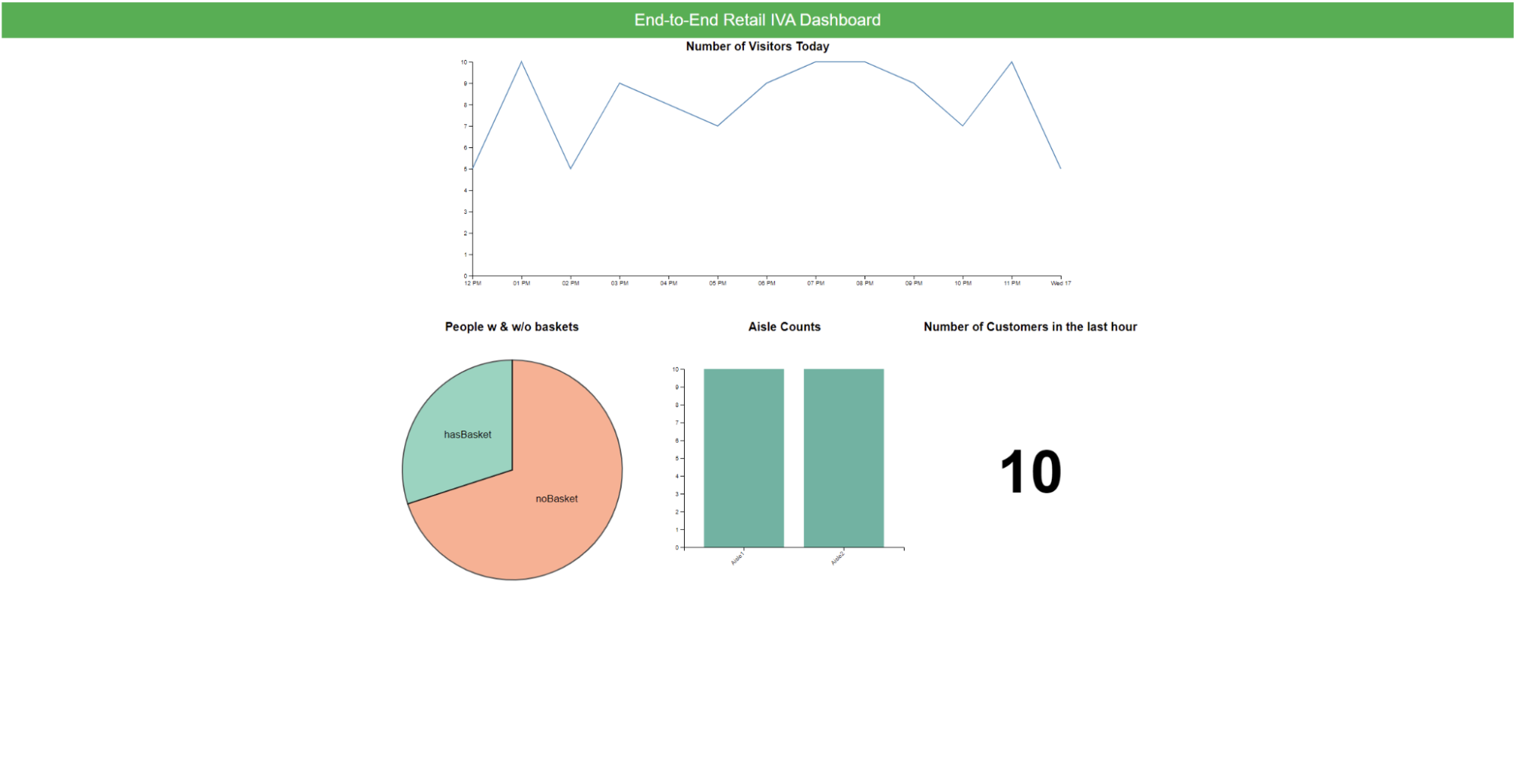
A dashboard with a line graph to track the number of visitors in a day, a pie chart with the ratio of customers with basket and without baskets, a bar graph with the number of customers in each aisle, and a number to depict the number of visitors in the last hour.
Figure 1. Frontend dashboard to visualize inference data

Introduction to the application architecture

Before diving into the detailed workflow, this section provides an overview of the tools that will be used to build this project. 

NVIDIA DeepStream SDK

NVIDIA DeepStream SDK is NVIDIA’s streaming analytics toolkit that enables GPU-accelerated video analytics with support for high-performance AI inference across a variety of hardware platforms. DeepStream includes several reference applications to jumpstart development. These reference apps can be easily modified to suit new use cases and are available inside the DeepStream Docker images and at deepstream_reference_apps on GitHub. 

This retail vision AI application is built on top of two of the reference applications, ­deepstream-test4 and deepstream-test5. Figure 2 shows the architecture of a typical DeepStream application.
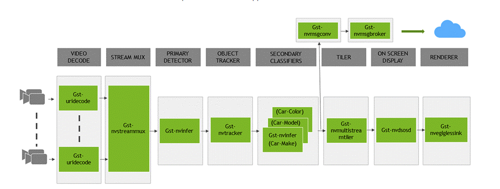
Graphic showing a DeepStream reference architecture workflow, including Video Decoding, Stream Mux, Primary Detector, Object Tracker, Secondary Classifiers, Tiler, On-Screen Display, and Renderer.
Figure 2. NVIDIA DeepStream reference application architecture

NVIDIA TAO Toolkit and pretrained models 

NVIDIA TAO (Train, Adapt, and Optimize) Toolkit enables fine-tuning a variety of AI pretrained models to new domains. The TAO Toolkit is used in concert with the DeepStream application to perform analyses for unique use cases. 

In this project, the model is used to detect whether or not a customer is carrying a shopping basket. DeepStream enables a seamless integration of TAO Toolkit with its existing pipeline without the need for heavy configuration. 

Getting started with TAO Toolkit is easy. TAO Toolkit provides complete Jupyter notebooks for model customization for 100+ combinations of CV architectures and backbones. TAO Toolkit also provides a library of task-specific pretrained models for common retail tasks like people detection, pose estimation, action recognition, and more. To get started, see TAO Toolkit Quick Start

Retail vision AI application workflow

The retail vision AI application architecture (Figure 3) consists of the following stages:

A DeepStream Pipeline with the following configuration:

  • Primary Detector: Configure PeopleNet pretrained model from NGC to detect ‘Persons’
  • Secondary Detector: Custom classification model trained using the TAO Toolkit for shopping basket detection
  • Object Tracker: NvDCF tracker (in the accuracy configuration) to track the movement in the video stream
  • Message Converter: Message converter to generate custom Kafka streaming payload from inference data
  • Message Broker: Message broker to relay inference data to a Kafka receiver

kSQL Time Series Database: Used to store inference output streams from an edge inference server

Django Web Application: Application to analyze data stored in the kSQL database to generate insights regarding store performance, and serve these metrics as RESTful APIs and a web dashboard
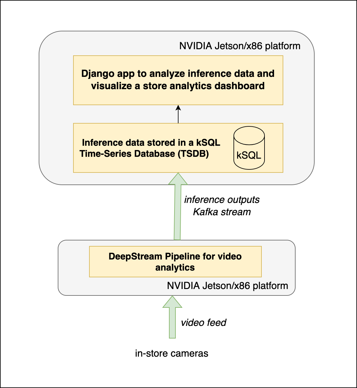
The architectural diagram for retail vision AI, including the workflow from taking the input from in-store cameras as the video feed and using the DeepStream pipeline for the video analytics. This is followed by the Inference in a kSQL Time Series Database (TSDB) and then transferred to the Django App where the Dashboard is created.
Figure 3. Retail vision AI application architecture

Additionally, this app is built for x86 platforms with an NVIDIA GPU. However, it can be easily deployed on NVIDIA Jetson embedded platforms, such as the NVIDIA Jetson AGX Orin. 

The next section walks you through the steps involved in building the application. 

Step 1: Building a custom NVIDIA DeepStream pipeline 

To build the retail data analytics pipeline, start with the NVIDIA DeepStream reference applications deepstream-test4 and deepstream-test5. Code for the pipeline and a detailed description of the process is available in the deepstream-retail-analytics GitHub repo. We recommend using this post as a walkthrough to the code in the repository.

The deepstream-test4 application is a reference DeepStream pipeline that demonstrates adding custom-detected objects as NVDS_EVENT_MSG_META user metadata and attaching it to the buffer to be published. The deepstream-test5 is an end-to-end app that demonstrates how to use nvmsgconv and nvmsgbroker plugins in multistream pipelines, create NVDS_META_EVENT_MSG type of meta, and stream inference outputs using Kafka and other sink types. 

This pipeline also integrates a secondary classifier in addition to the primary object detector, which can be useful for detecting shopper attributes once a person is detected in the retail video analytics application. The test4 application is used to modify the nvmsgconv plugin to include retail analytics attributes. Then, refer to the test5 application for secondary classifiers and streaming data from the pipeline using the nvmsgbroker over a Kafka topic. 

Since the first step of the workflow is to identify persons and objects from the video feed, start by using the deepstream-test4 application for primary object detection. This object detection is done on the PeopleNet pretrained model that, by default, takes video input and detects people or their belongings.

For this use case, configure the model to capture only information about people. This can be accomplished easily by storing information only about the subset of frames that contain a person in the dataset.

With the primary person object detection done, use deepstream-test5 to add a secondary object classification model. This object classification shows whether or not a detected person is carrying a basket.

Step 2: Building a custom model for shopping basket detection with NVIDIA TAO Toolkit

This section shows how to use the TAO Toolkit to fine-tune an object classification model and find out whether a person detected in the PeopleNet model is carrying a shopping basket (Figure 4). 
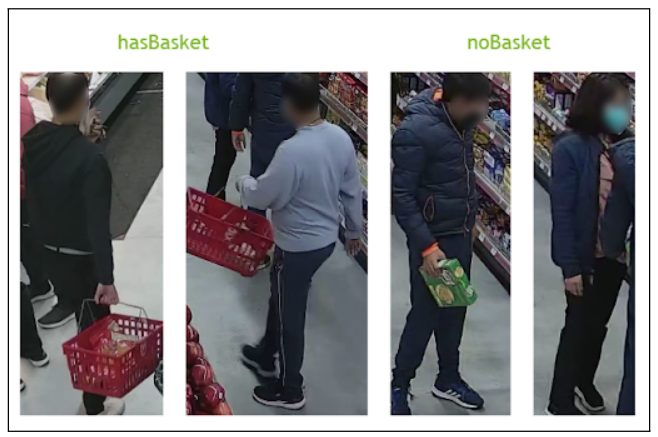
The sample image classifier files where you can see the customers in the ‘hasBasket’ category are clearly carrying shopping baskets. The second category of ‘noBasket’ shows customers without baskets in their hands.
Figure 4. Shoppers classified to have baskets (left) and not to have baskets (right)

To get started, collect and annotate training data from a retail environment for performing object classification. Use the Computer Vision Annotation Tool (CVAT) to annotate persons observed with the following labels:

  • hasBasket: Person is carrying a basket
  • noBasket: Person is not carrying a basket

This annotation is stored as a KITTI formatted dataset, where each line corresponds to a frame and thus an object. To make the data compatible for object classification, use the sample ‘kitti_to_classification‘ Python file on GitHub to crop the dataset. You can then perform object classification on it.

Next, use the TAO Toolkit to fine-tune a Resnet34 image classification model to perform classification on the training data. Learn more about the fine-tuning process at deepstream-retail-analytics/tree/main/TAO on GitHub.

After the custom model is created, run inference to validate that the model works as expected.

Step 3: Integrating the Kafka message broker to create a custom frontend dashboard

With the primary object detection and secondary object classification models ready, the DeepStream application needs to relay this inference data to an analytics web server. Use the deepstream-test5 reference application as a template to stream data using Apache Kafka. 

Here, a Kafka adapter that is built into DeepStream is used to publish messages to the Kafka message broker. Once the web server receives the Kafka streams from each camera inside a store, these inference output data are stored in a kSQL time-series database.

DeepStream has a default Kafka messaging shared library object that enables users to perform primary object detection and transmit the data seamlessly. This project further modifies this library to include information about the secondary classifier as well. This helps to stream data about shopping basket use inside the store.

The current DeepStream library includes NvDsPersonObject, which is used to define the persons detected in the primary detector. To ensure that the basket detection is mapped to each person uniquely, modify this class to include a hasBasket attribute in addition to the previously present attributes. Find more details at deepstream-retail-analytics/tree/main/nvmsgconv on GitHub.

After modifying the NvDsPersonObject to include basket detection, use the pipeline shown in Figure 5 to ensure the functionality for basket detection works appropriately.

The Application pipeline, which walks through all the steps in the workflow starting from video source and h264-parser, followed by nvh264-decoder, nvstreammux, the nvinfer primary detector, the nvtracker, nvinfer for secondary detection, nvvidconv, nvsod and then the tee which branches to msgconv, nveglglessink, msgconv, and msgbroker.
Figure 5. Retail vision AI application pipeline

As shown in the application pipeline in Figure 5, object detection and tracking are performed with the help of pgie and sgie. These are part of the nvinfer plugin as the primary and secondary inference engines. With nvtracker, transfer the data to the nvosd plugin. This nvosd plugin is responsible for drawing boxes around the objects that were detected in the previous sections.

Next, this inference data needs to be converted into message payload based on a specific schema that can be later consumed by the Kafka message broker to store and analyze the results. Use the NvDsPersonsObject (generated previously) for the updated payload in the eventmsg_payload file.

Finally, you now have the message payload with the custom schema. Use this to pass it through the Kafka protocol adapter and publish messages that the DeepStream application sends to the Kafka message broker at the specified broker address and topic. At this point, the final message payload is ready.

Now that the DeepStream pipeline is ready, build a web application to store the streaming inference data into a kSQL database. This web app, built using the Django framework, analyzes the inference data to generate metrics regarding store performance discussed earlier. These metrics are available through a RESTful API documented at deepstream-retail-analytics/tree/main/ds-retail-iva-frontend on GitHub. 

To demonstrate the API functionality, we built a frontend web dashboard to visualize the results of the analytics server. This dashboard acts as a template for a storewide analytics system. 

Results

The previous steps demonstrated how to easily develop an end-to-end retail video analytics pipeline using NVIDIA DeepStream and NVIDIA TAO Toolkit. This pipeline helps retail establishments capitalize on pre-existing video feeds and find insightful information they can use to improve profits. 

The workflow culminates in an easy-to-use web dashboard to analyze invaluable storewide data in real time. As shown in Figure 1, the dashboard presents the following information:

  • Number of store visitors throughout the day
  • Information about the proportion of customers shopping with and without baskets
  • Visitors counts per store aisle
  • Store occupancy heatmaps
  • Customer journey visualization

These attributes can be easily amended to include information about specific use cases that are more relevant to each individual store. Stores can use this information to schedule staffing and improve the store layout to maximize efficiency. 

For example, Figure 6 shows the overall distribution of customers in the store throughout the day, as well as the ratio of customers with and without baskets, respectively. While this sample application supports only a single camera stream, it can be easily modified to support multiple cameras. Scaling this application to multiple stores is equally easy to do. 

A figure displaying the number of customers in the store over time as a bar graph with many rows and different distribution throughout the x-axis (left). On the right side, the  pie chart depicts the ratio of customers who have ‘noBasket’ with respect to the customers who fall into the ‘hasBasket’ category. There are 82.6% customers who have ‘noBasket’ vs 17.4% who are in the ‘hasBasket’ category.
Figure 6. Inference data for the number of customers in the store over time (left) and the ratio of customers with baskets to those without baskets (right)

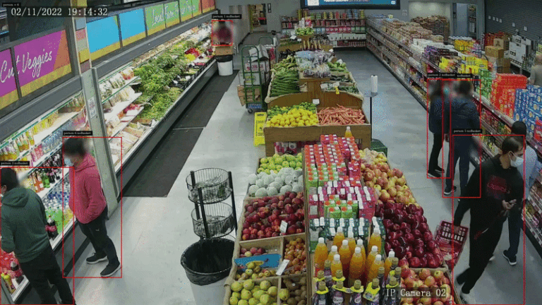
The application uniquely detects person 11 carrying the shopping basket by setting the attribute of hasBasket, whereas the other customers who do not carry the basket are marked with noBasket. Additionally, the person 1 with a cardboard box is not identified to have a basket. Thus, the model is robust against false positives, ensuring that it was successfully trained to only pick up relevant information for this use case.

Summary 

This post demonstrated an end-to-end process to develop a vision AI application to perform retail analytics using NVIDIA TAO Toolkit and NVIDIA DeepStream SDK. Retail establishments can use the flux of video data they already have and build state-of-the-art video analytics applications. These apps can be deployed in real time and require minimal configuration to get started. In addition, the high customizability of this application ensures that it can be applied to any use case a store might benefit from.

Get started using the sample deepstream-retail-analytics application on GitHub.

Categories
Offsites

Formation of Robust Bound States of Interacting Photons

When quantum computers were first proposed, they were hoped to be a way to better understand the quantum world. With a so-called “quantum simulator,” one could engineer a quantum computer to investigate how various quantum phenomena arise, including those that are intractable to simulate with a classical computer.

But making a useful quantum simulator has been a challenge. Until now, quantum simulations with superconducting qubits have predominantly been used to verify pre-existing theoretical predictions and have rarely explored or discovered new phenomena. Only a few experiments with trapped ions or cold atoms have revealed new insights. Superconducting qubits, even though they are one of the main candidates for universal quantum computing and have demonstrated computational capabilities beyond classical reach, have so far not delivered on their potential for discovery.

In “Formation of Robust Bound States of Interacting Photons”, published in Nature, we describe a previously unpredicted phenomenon first discovered through experimental investigation. First, we present the experimental confirmation of the theoretical prediction of the existence of a composite particle of interacting photons, or a bound state, using the Google Sycamore quantum processor. Second, while studying this system, we discovered that even though one might guess the bound states to be fragile, they remain robust to perturbations that we expected to have otherwise destroyed them. Not only does this open the possibility of designing systems that leverage interactions between photons, it also marks a step forward in the use of superconducting quantum processors to make new scientific discoveries by simulating non-equilibrium quantum dynamics.

Overview

Photons, or quanta of electromagnetic radiation like light and microwaves, typically don’t interact. For example, two intersecting flashlight beams will pass through one another undisturbed. In many applications, like telecommunications, the weak interactions of photons is a valuable feature. For other applications, such as computers based on light, the lack of interactions between photons is a shortcoming.

In a quantum processor, the qubits host microwave photons, which can be made to interact through two-qubit operations. This allows us to simulate the XXZ model, which describes the behavior of interacting photons. Importantly, this is one of the few examples of integrable models, i.e., one with a high degree of symmetry, which greatly reduces its complexity. When we implement the XXZ model on the Sycamore processor, we observe something striking: the interactions force the photons into bundles known as bound states.

Using this well-understood model as a starting point, we then push the study into a less-understood regime. We break the high level of symmetries displayed in the XXZ model by adding extra sites that can be occupied by the photons, making the system no longer integrable. While this nonintegrable regime is expected to exhibit chaotic behavior where bound states dissolve into their usual, solitary selves, we instead find that they survive!

Bound Photons

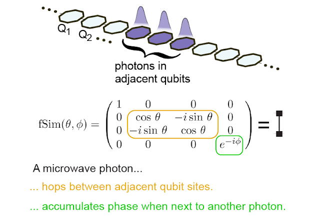
To engineer a system that can support the formation of bound states, we study a ring of superconducting qubits that host microwave photons. If a photon is present, the value of the qubit is “1”, and if not, the value is “0”. Through the so-called “fSim” quantum gate, we connect neighboring sites, allowing the photons to hop around and interact with other photons on the nearest-neighboring sites.

Superconducting qubits can be occupied or unoccupied with microwave photons. The “fSim” gate operation allows photons to hop and interact with each other. The corresponding unitary evolution has a hopping term between two sites (orange) and an interaction term corresponding to an added phase when two adjacent sites are occupied by a photon.
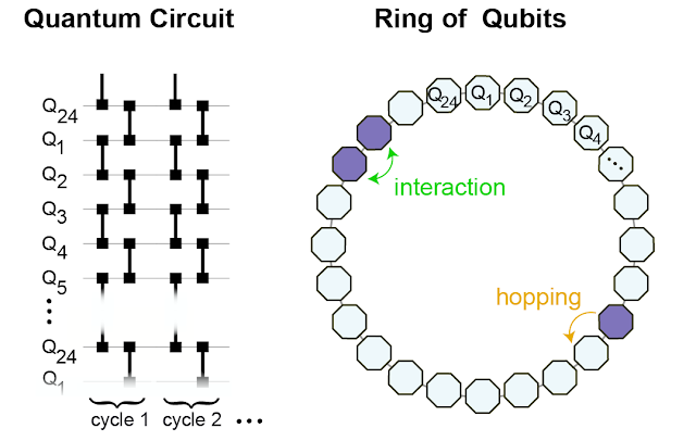
We implement the fSim gate between neighboring qubits (left) to effectively form a ring of 24 interconnected qubits on which we simulate the behavior of the interacting photons (right).

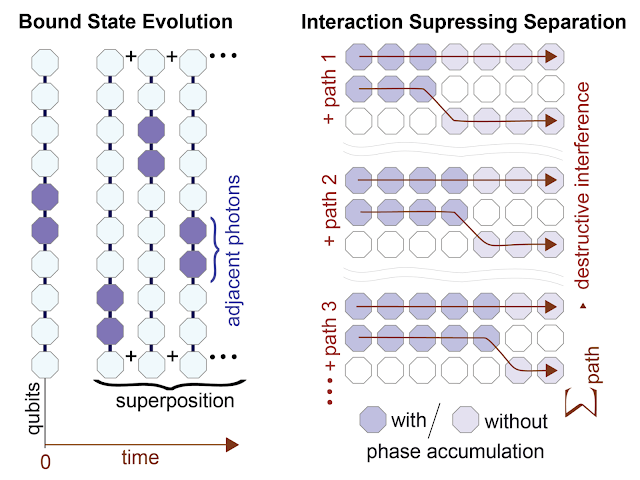
The interactions between the photons affect their so-called “phase.” This phase keeps track of the oscillation of the photon’s wavefunction. When the photons are non-interacting, their phase accumulation is rather uninteresting. Like a well-rehearsed choir, they’re all in sync with one another. In this case, a photon that was initially next to another photon can hop away from its neighbor without getting out of sync. Just as every person in the choir contributes to the song, every possible path the photon can take contributes to the photon’s overall wavefunction. A group of photons initially clustered on neighboring sites will evolve into a superposition of all possible paths each photon might have taken.

When photons interact with their neighbors, this is no longer the case. If one photon hops away from its neighbor, its rate of phase accumulation changes, becoming out of sync with its neighbors. All paths in which the photons split apart overlap, leading to destructive interference. It would be like each choir member singing at their own pace — the song itself gets washed out, becoming impossible to discern through the din of the individual singers. Among all the possible configuration paths, the only possible scenario that survives is the configuration in which all photons remain clustered together in a bound state. This is why interaction can enhance and lead to the formation of a bound state: by suppressing all other possibilities in which photons are not bound together.

Left: Evolution of interacting photons forming a bound state. Right: Time goes from left to right, each path represents one of the paths that can break the 2-photon bonded state. Due to interactions, these paths interfere destructively, preventing the photons from splitting apart.
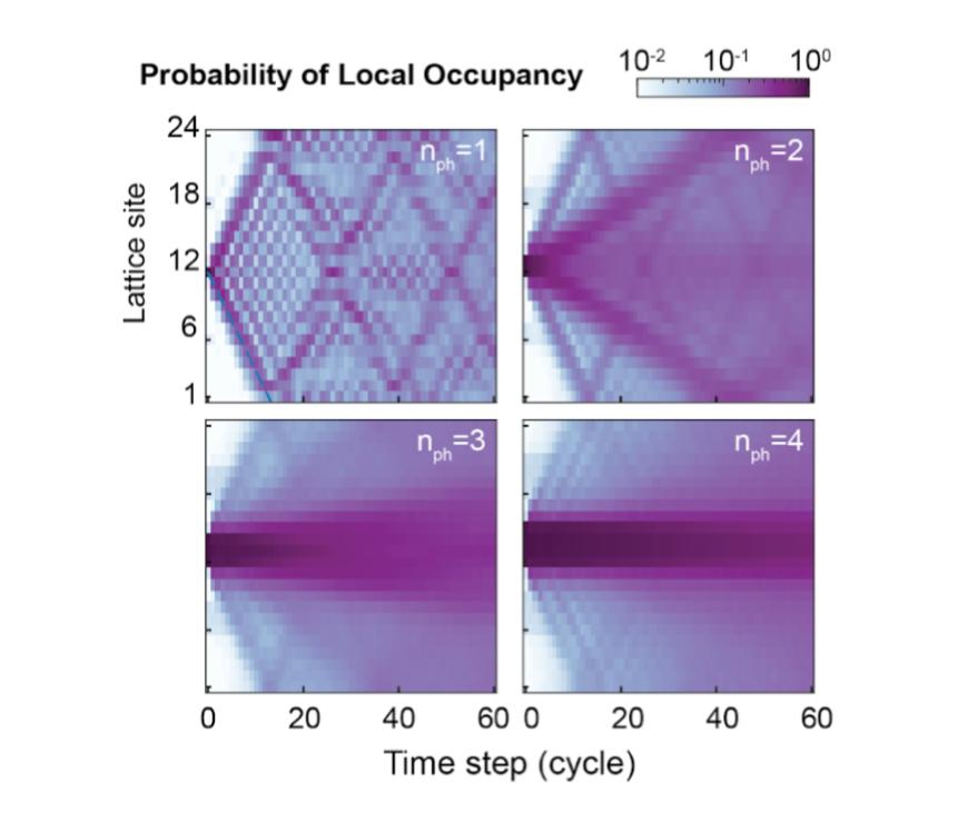
Occupation probability versus gate cycle, or discrete time step, for n-photon bound states. We prepare bound states of varying sizes and watch them evolve. We observe that the majority of the photons (darker colors) remain bound together.

In our processor, we start by putting two to five photons on adjacent sites (i.e., initializing two to five adjacent qubits in “1”, and the remaining qubits in “0”), and then study how they propagate. First, we notice that in the theoretically predicted parameter regime, they remain stuck together. Next, we find that the larger bound states move more slowly around the ring, consistent with the fact that they are “heavier”. This can be seen in the plot above where the lattice sites closest to Site 12, the initial position of the photons, remain darker than the others with increasing number of photons (nph) in the bound state, indicating that with more photons bound together there is less propagation around the ring.

Bound States Behave Like Single Composite Particles

To more rigorously show that the bound states indeed behave as single particles with well-defined physical properties, we devise a method to measure how the energy of the particles changes with momentum, i.e., the energy-momentum dispersion relation.

To measure the energy of the bound state, we use the fact that the energy difference between two states determines how fast their relative phase grows with time. Hence, we prepare the bound state in a superposition with the state that has no photons, and measure their phase difference as a function of time and space. Then, to convert the result of this measurement to a dispersion relation, we utilize a Fourier transform, which translates position and time into momentum and energy, respectively. We’re left with the familiar energy-momentum relationship of excitations in a lattice.

Spectroscopy of bound states. We compare the phase accumulation of an n-photon bound state with that of the vacuum (no photons) as a function of lattice site and time. A 2D Fourier transform yields the dispersion relation of the bound-state quasiparticle.

Breaking Integrability

The above system is “integrable,” meaning that it has a sufficient number of conserved quantities that its dynamics are constrained to a small part of the available computational space. In such integrable regimes, the appearance of bound states is not that surprising. In fact, bound states in similar systems were predicted in 2012, then observed in 2013. However, these bound states are fragile and their existence is usually thought to derive from integrability. For more complex systems, there is less symmetry and integrability is quickly lost. Our initial idea was to probe how these bound states disappear as we break integrability to better understand their rigidity.

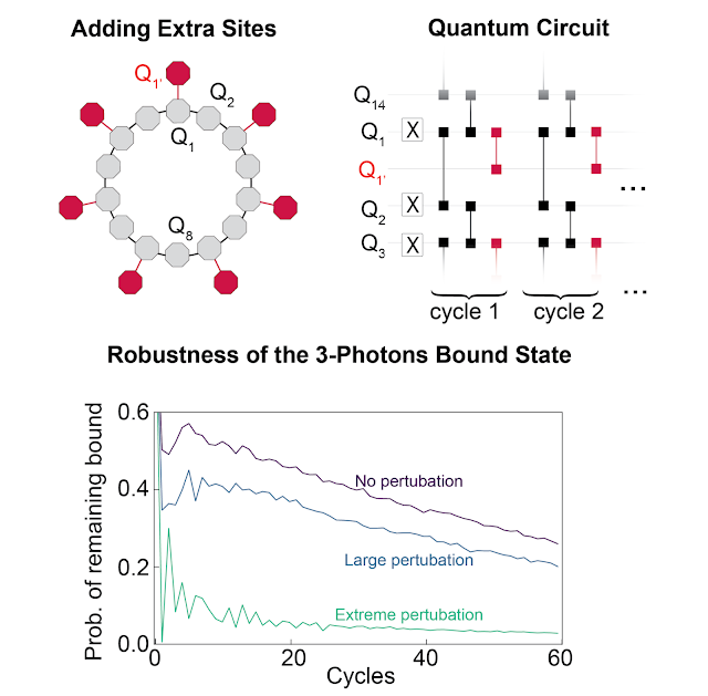
To break integrability, we modify which qubits are connected with fSim gates. We add qubits so that at alternating sites, in addition to hopping to each of its two nearest-neighboring sites, a photon can also hop to a third site oriented radially outward from the ring.

While a bound state is constrained to a very small part of phase space, we expected that the chaotic behavior associated with integrability breaking would allow the system to explore the phase space more freely. This would cause the bound states to break apart. We find that this is not the case. Even when the integrability breaking is so strong that the photons are equally likely to hop to the third site as they are to hop to either of the two adjacent ring sites, the bound state remains intact, up to the decoherence effect that makes them slowly decay (see paper for details).

Top: New geometry to break integrability. Alternating sites are connected to a third site oriented radially outward. This increases the complexity of the system, and allows for potentially chaotic behavior. Bottom: Despite this added complexity pushing the system beyond integrability, we find that the 3-photon bound state remains stable even for a relatively large perturbation. The probability of remaining bound decreases slowly due to decoherence (see paper).

Conclusion

We don’t yet have a satisfying explanation for this unexpected resilience. We speculate that it may be related to a phenomenon called prethermalization, where incommensurate energy scales in the system can prevent a system from reaching thermal equilibrium as quickly as it otherwise would. We believe further investigations will hopefully lead to new insights into many-body quantum physics, including the interplay of prethermalization and integrability.

Acknowledgements

We would like to thank our Quantum Science Communicator Katherine McCormick for her help writing this blog post.

Categories
Misc

Boosting Dynamic Programming Performance Using NVIDIA Hopper GPU DPX Instructions

Dynamic programming (DP) is a well-known algorithmic technique and a mathematical optimization that has been used for several decades to solve groundbreaking…
Dynamic programming (DP) is a well-known algorithmic technique and a mathematical optimization that has been used for several decades to solve groundbreaking problems in computer science.

An example DP use case is route optimization with hundreds or thousands of constraints or weights using the Floyd-Warshall all-pair shortest paths algorithm. Another use case is the alignment of reads for genome sequence alignment using the Needleman-Wunsch or Smith-Waterman algorithms.

NVIDIA Hopper GPU Dynamic Programming X (DPX) instructions accelerate a large class of dynamic programming algorithms used in areas such as genomics, proteomics, and robot path planning. Accelerating these dynamic programming algorithms can help researchers, scientists, and practitioners glean insights much faster about the underlying DNA or protein structures and several other areas.

What is dynamic programming?

DP techniques initially involve expressing the algorithm recursively, where the larger problem is broken down into subproblems that are easier to solve.

A common computational optimization used in DP is to save the results of the subproblems and use them in subsequent steps of the problem, instead of recomputing the solution each time. This step is called memoization. Memoization facilitates avoiding the recursion steps and instead enables using an iterative, look-up, tablebased formulation. The previously computed results are stored in the look-up table.

One of the key observations in many DP problems is that the solution to a larger problem often involves computing the minimum or maximum of the previously computed solutions. The larger problem’s solution is within a delta of that min-max of previous solutions.

DP techniques, in general, achieve the same results as brute force algorithms, but with dramatic reductions in the computational requirements and execution times.

DP example: Accelerating the Smith-Waterman algorithm

NVIDIA Clara Parabricks is a GPU-accelerated genomic analysis suite of tools that heavily uses the Smith-Waterman algorithm and runs on NVIDIA GPUs: A100, V100, A40, A30, A10, A6000, T4, and soon the newest H100.

Genome sequencing has fundamental applications with universal benefits, with examples that include personalized medicine or tracking disease spread. Every cell in living organisms encodes genetic information using a sequence of four nucleotides in DNA (or bases). The nucleotides are adenine, cytosine, guanine, and thymine, represented by A, C, T, and G.

Simple organisms like viruses have a sequence of 10–100K bases while human DNA consists of about three billion base pairs. There are instruments (chemical– or electrical-signal–based) that sequence the bases of short segments of genetic material, called reads. These reads are typically 100–100K bases long, depending on the sequencer technology used for gathering the reads.

A critical computational step in genome sequence analysis is to align the reads to find the best match among a pair of reads. These reads can be 100-400 base pairs long in second-generation sequencers, and up to 100K bases long in third-generation sequencers. Aligning reads is a computational step that is repeated tens or hundreds of millions of times.

There are challenges in finding the best match that include the following:

  • Naturally occurring variations in genomes that give organisms within a species their specific traits
  • Errors in the reads themselves resulting from the sequencing instrument or underlying chemical processes

The best match between a pair of reads is equivalent to an approximate string match between a pair of strings with steps that reward matches and penalize differences. The differences between the reads could be mismatches, insertions, or deletions.

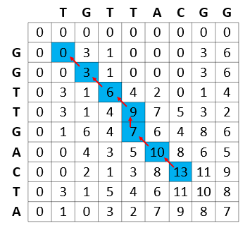
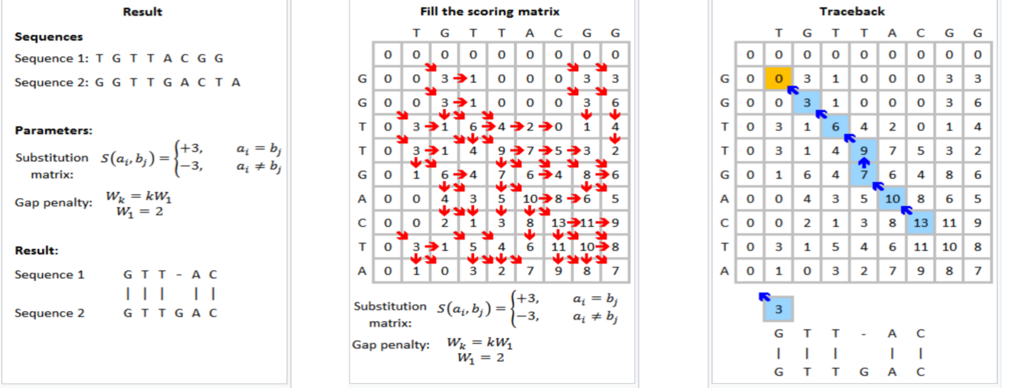
The Smith-Waterman algorithm proceeds to find the best match between a pair of sequences TGTTACGG and GGTTGACTA.
Figure 1. Smith-Waterman scoring matrix and traceback for a pair of sequences (Source: Wikipedia)

Figure 1 shows that the Smith-Waterman step in genomic sequencing aims to find the best match between the read sequences TGTTACGG and GGTTGACTA. The resulting best match is shown to be GTT-AC (from sequence 1, the “-” representing a deletion) with GTTGAC (from sequence 2). The scoring scheme in each step rewards matches (+3), penalizes mismatches (-3), and penalizes insertions and deletions (see the gap penalty formula in Figure 1).

This is an example formulation of the Smith-Waterman algorithm. Implementers of the Smith-Waterman algorithm are allowed to customize the rewards and penalties.

While computing the best match between TGTTACGG and GGTTGACTA, the Smith-Waterman algorithm also computes the best matches for all prefixes of TGTTACGG with all prefixes of GGTTGACTA. It proceeds from the start of these sequences and uses the results of the smaller prefixes to feed into the problem of finding the solution for the larger prefixes.

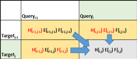
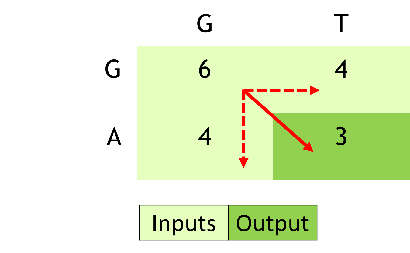
Diagram shows a simplified cell calculation step between GA and GT. Only the cell entry for A versus T has to be calculated. This is a mismatch. Take the maximum score after accounting for substitution and gap penalties.
Figure 2. A simplified cell calculation step in the Smith-Waterman algorithm

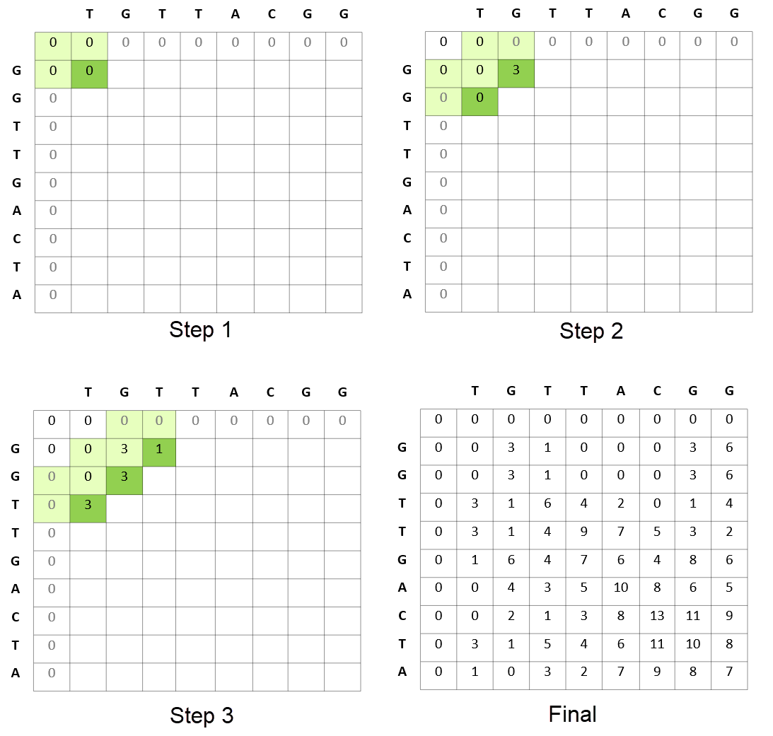
Figure 3 shows how the algorithm proceeds in terms of calculating the scores of matrices for matching a sequence of reads. This comparative matching is the computationally expensive step of the Smith-Waterman algorithm.

This is just one of the formulations of how the Smith-Waterman algorithm proceeds. Different formulations can result in the algorithm proceeding row-wise or column-wise as examples.

Each cell calculation requires the cell to the top, left, and top-left to be available. This diagram shows a formulation of Smith-Waterman that proceeds diagonally, starting from the top-left corner of the scoring matrix.
Figure 3. Example steps of the Smith-Waterman algorithm

After the score matrix is computed, the next step involves backtracking from the highest score to the origin of each of these scores. This is a computationally light step given that each cell maintains how it got its score (the source cell for score calculation).

If each cell keeps a tab of where the score was derived from (top, left, top-left), tracking back the score to a zero will show the best match(es) between the sequences.
Figure 4. Backtracking from the highest score in the Smith-Waterman algorithm

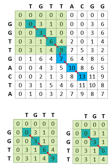
Figure 5 shows the computational efficiency of the Smith-Waterman calculations, where each of the subproblems solved by the algorithm is stored in the result matrix and never recomputed.

For example, in the process of calculating the best match of GGTTGACTA and TGTTACGG, the Smith-Waterman algorithm reuses the best match between GGTT (prefix of GGTTGACTA) and TGTT (prefix of TGTTACGG). In turn, while calculating the best match of GGTT and TGTT, the best match of all prefixes of these strings are calculated and reused (for example, best match of GGTT and TGT).

The best match of GGTT with TGTT also calculates the best match of GGTT with TGT. In fact, the best match with every prefix of TGTTACGG with every prefix of GGTTGACTA is calculated in the scoring matrix.
Figure 5. Subproblems solved by the Smith-Waterman algorithm

Leveraging DPX instructions for better performance

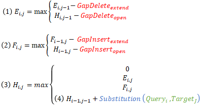
 The inner loop in a real Smith-Waterman implementation involves the following for each cell:

  • Updating deletion penalties
  • Updating insertion penalties
  • Updating the score based on the updated insertion and deletion penalties.
Equations for the insertion and deletion penalties.
Practical implementations of Smith-Waterman must keep tabs of the insertion and deletion penalties in addition to the scores.
Figure 6. Updating insertion penalty, deletion penalties, and scores in a Smith-Waterman implementation step

The NVIDIA Hopper Architecture math API provides dramatic acceleration for such calculations. The APIs expose the acceleration provided by NVIDIA Hopper Streaming Multiprocessor for additions followed by minimum or maximum as a fused operation (for example, __viaddmin_s16x2_relu, an intrinsic that performs per-halfword max(min(a + b, c), 0)).

Another example of an API that is extensively leveraged by Smith-Waterman software is a three-way min or max followed by a clamp to zero ( for example, __vimax3_s16x2_relu, an intrinsic that performs per-halfword max(max(max(a, b), c), 0)).

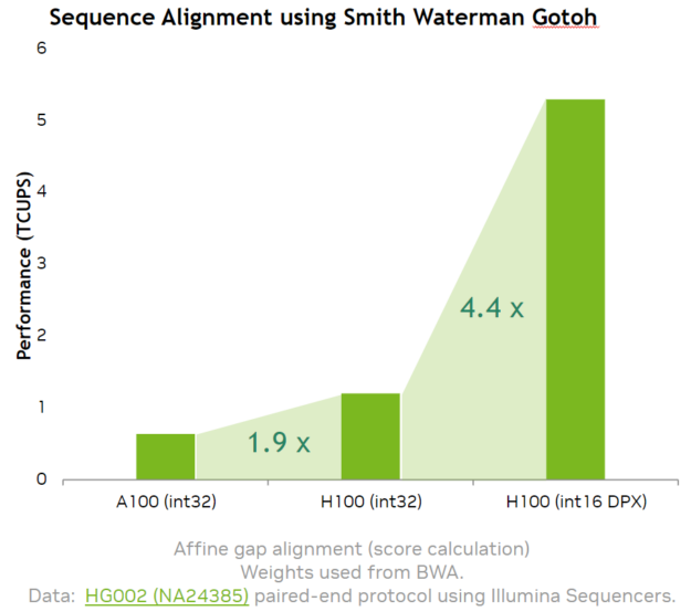
Our implementation of the Smith-Waterman algorithm using the NVIDIA Hopper DPX instruction math APIs provides a 7.8x speedup over A100.

NVIDIA Hopper DPX instructions enable over a 7x speedup for the Smith-Waterman score matrix calculations.
Figure 7. Smith-Waterman calculations speedup using DPX instructions in H100

Needleman-Wunsch and partial order alignment

In the same way that Smith-Waterman algorithms use DPX instructions, there is a large family of alignment algorithms that essentially use the same principles.

Examples include the Needleman-Wunsch algorithm in which the basic flow of the algorithm resembles the Smith-Waterman closely. However, the initialization, insertion, and gap penalties are calculated differently between these two approaches.

Algorithms like Partial Order Alignment make dense use of cell calculations that closely resemble Smith-Waterman cell calculations in their inner loop.

All-pair shortest paths

Robotic path planning with thousands or tens of thousands of objects is a common problem in warehouses where the environment is dynamic with many moving objects. These scenarios can involve dynamic replanning every few milliseconds.

The inner loop of most all-pair shortest paths algorithms is as shown using the following Floyd-Warshall algorithm example. The pseudocode shows how the all-pair shortest paths algorithm has an inner loop that updates the min distance between each vertex pair. The most-dense operation is essentially an add followed by a min operation.

initialize(dist); # initialize nearest neighbors to actual distance, all others = infinity 
for k in range(V): #order of visiting k values not important, must visit each value

	# pick all vertices as source in parallel
	Parallel for_each i in range(V):

		# Pick all vertices as destinations for the
		# above picked source
		Parallel for_each j in range(V):

			# If vertex k is on the shortest path from
			# i to j, then update the value of dist[i][j]
			dist[i][j] = min (dist[i][j], dist[i][j] + dist[k][j])

			# dist[i][j] calculation can be parallel within each k
			# All dist[i][j] for a single ‘k’ must be computed 
                        # before moving to the next ‘k’
		Synchronize

The speedup offered by DPX instructions makes it possible to dramatically scale the number of objects analyzed or have the re-optimization done in real time with fewer GPUs and optimal results.

Accelerate dynamic programming algorithms with DPX instructions 

Using NVIDIA Hopper DPX instructions demonstrated speedups of up to 7.8x on the A100 GPU for Smith-Waterman, which is key in many genomic sequence alignment and variant calling applications. The exposure in math APIs, available in CUDA 12, enables the configurable implementation of the Smith-Waterman algorithm to suit different user needs, as well as algorithms like Needleman-Wunsch.

DPX instructions accelerate a large class of dynamic programming algorithms such as DNA or protein sequencing, and robot path planning. Most importantly, these algorithms can lead to dramatic speed-ups in disease diagnosis, drug discoveries, and robot autonomy, making our everyday lives better.

Acknowledgments

We’d like to thank Bill Dally, Alejandro Cachon, Mehrzad Samadi, Shirish Gadre, Daniel Stiffler, Rob Van der Wijngaart, Joseph Sullivan, Nikita Astafev, Seamus O’Boyle, and many others across NVIDIA.

Categories
Misc

What Is a Pretrained AI Model?

Imagine trying to teach a toddler what a unicorn is. A good place to start might be by showing the child images of the creature and describing its unique features. Now imagine trying to teach an artificially intelligent machine what a unicorn is. Where would one even begin? Pretrained AI models offer a solution. A Read article >

The post What Is a Pretrained AI Model? appeared first on NVIDIA Blog.

Categories
Misc

The Hunt Is On: ‘The Witcher 3: Wild Hunt’ Next-Gen Update Coming to GeForce NOW

It’s a wild GFN Thursday — The Witcher 3: Wild Hunt next-gen update will stream on GeForce NOW day and date, starting next week. Today, members can stream new seasons of Fortnite and Genshin Impact, alongside eight new games joining the library. In addition, the newest GeForce NOW app is rolling out this week with Read article >

The post The Hunt Is On: ‘The Witcher 3: Wild Hunt’ Next-Gen Update Coming to GeForce NOW appeared first on NVIDIA Blog.

Categories
Misc

‘23 and AV: Transportation Industry to Drive Into Metaverse, Cloud Technologies

As the autonomous vehicle industry enters the next year, it will start navigating into even greater technology frontiers. Next-generation vehicles won’t just be defined by autonomous driving capabilities. Everything from the design and production process to the in-vehicle experience is entering a new era of digitization, efficiency, safety and intelligence. These trends arrive after a Read article >

The post ‘23 and AV: Transportation Industry to Drive Into Metaverse, Cloud Technologies appeared first on NVIDIA Blog.

Categories
Misc

Qubit Pharmaceuticals Accelerates Drug Discovery With Hybrid Quantum Computing

The promise of quantum computing is to solve unsolvable problems. And companies are already making headway with hybrid approaches — those that combine classical and quantum computing — to tackle challenges like drug discovery for incurable diseases. By accelerating drug molecule simulation and modeling with hybrid quantum computing, startup Qubit Pharmaceuticals is significantly reducing the Read article >

The post Qubit Pharmaceuticals Accelerates Drug Discovery With Hybrid Quantum Computing appeared first on NVIDIA Blog.

Categories
Misc

GFN Thursday Dashes Into December With 22 New Games, Including ‘Marvel Midnight Suns’ Streaming Soon

It’s a new month, which means GeForce NOW’s got the list of 22 new games arriving in December. Rise up for Marvel’s Midnight Suns, from publisher 2K Games, streaming on GeForce NOW later this month. Then get ready to move out, members. Battlefield 2042 is the latest game from the Electronic Arts catalog streaming on Read article >

The post GFN Thursday Dashes Into December With 22 New Games, Including ‘Marvel Midnight Suns’ Streaming Soon appeared first on NVIDIA Blog.

Categories
Misc

Cheers to AI: Monarch Tractor Launches First Commercially Available Electric, ‘Driver Optional’ Smart Tractor

Livermore, Calif., renowned for research and vineyards, is plowing in a new distinction: the birthplace of the first commercially available smart tractor. Local startup Monarch Tractor has announced the first of six Founder Series MK-V tractors are rolling off the production line at its headquarters. Constellation Brands, a leading wine and spirits producer and beer Read article >

The post Cheers to AI: Monarch Tractor Launches First Commercially Available Electric, ‘Driver Optional’ Smart Tractor appeared first on NVIDIA Blog.

Categories
Misc

Meet the Omnivore: Cloud Architect Takes Infrastructure Visualization to New Heights With NVIDIA Omniverse

As a Microsoft Certified Azure cloud specialist and DevOps automation engineer, Gavin Stevens is deeply in tune with cloud architect workflows.

The post Meet the Omnivore: Cloud Architect Takes Infrastructure Visualization to New Heights With NVIDIA Omniverse appeared first on NVIDIA Blog.