Categories
Misc

The Truck Stops Here: How AI Is Creating a New Kind of Commercial Vehicle

For many, the term “autonomous vehicles” conjures up images of self-driving cars. Autonomy, however, is transforming much more than personal transportation. Autonomous trucks are commercial vehicles that use AI to automate everything from shipping yard operations to long-haul deliveries. Due to industry pressures from rising delivery demand and driver shortages, as well as straightforward operational Read article >

The post The Truck Stops Here: How AI Is Creating a New Kind of Commercial Vehicle appeared first on The Official NVIDIA Blog.

Categories
Misc

Inception Spotlight: DarwinAI Achieves 96% Screening Accuracy for COVID-19 with Diverse CT Dataset

NVIDIA Inception partner DarwinAI developed a new AI model to detect COVID-19 in CT scans with 96% accuracy across a wide and diverse number of scenarios. The model, COVID-Net CT-2, was built using a number of large and diverse datasets created over several months with the University of Waterloo and is publicly available on GitHub.

Last year, the startup launched an open source neural network for COVID-19 detection called COVID-Net. Their new model builds upon the initiative with a more robust model, trained on the largest quantity and diversity of multinational patient cases in research literature. Their academic study detailing the construction and validation of the model can be found here.

DarwinAI used an NVIDIA RTX 6000 for training their neural network and the NVIDIA Jetson Nano embedded AI platform to run their inference workloads.

“By building COVID-NET CT-2 from such rich and voluminous data, we’ve been able to achieve a new level of screening accuracy, with COVID-19 sensitivity and positive predictive value exceeding 96% across a wide and diverse number of scenarios,” said Sheldon Fernandez, CEO of Darwin-AI. 

“Our XAI platform was instrumental in the construction of the original COVID-Net model. For this version, we have engaged two senior radiologists in Canada to validate the way in which COVID-Net CT-2 makes its decisions. Much to our delight, both confirmed the decision-making process of COVID-Net CT-2 is consistent with their own expert interpretations,” Fernandez added.  “In addition to illustrating the emerging cooperation between our respective domains, their validation exemplifies the importance of our XAI technology in constructing transparent and trustworthy AI.” 

The largest of the datasets used to develop the new AI model consists of over 4,500 patients across 15 countries with 200,000 CT slices.

Both DarwinAI and NVIDIA are enabling researchers to build neural networks to fight COVID-19 with the help of open source AI and publicly available pre-trained models. Medical imaging AI models for detecting COVID-19 in X-rays and CTs can be accessed through DarwinAI’s COVID-Net Initiative and the NVIDIA COVID-19 NGC Catalog.

Learn more about how AI, accelerated computing, and GPU technology are contributing to the worldwide battle against the novel coronavirus in the COVID-19 Research Hub.

Categories
Offsites

Machine Learning for Computer Architecture

One of the key contributors to recent machine learning (ML) advancements is the development of custom accelerators, such as Google TPUs and Edge TPUs, which significantly increase available compute power unlocking various capabilities such as AlphaGo, RankBrain, WaveNets, and Conversational Agents. This increase can lead to improved performance in neural network training and inference, enabling new possibilities in a broad range of applications, such as vision, language, understanding, and self-driving cars.

To sustain these advances, the hardware accelerator ecosystem must continue to innovate in architecture design and acclimate to rapidly evolving ML models and applications. This requires the evaluation of many different accelerator design points, each of which may not only improve the compute power, but also unravel a new capability. These design points are generally parameterized by a variety of hardware and software factors (e.g., memory capacity, number of compute units at different levels, parallelism, interconnection networks, pipelining, software mapping, etc.). This is a daunting optimization task, due to the fact that the search space is exponentially large1 while the objective function (e.g., lower latency and/or higher energy efficiency) is computationally expensive to evaluate through simulations or synthesis, making identification of feasible accelerator configurations challenging .

In “Apollo: Transferable Architecture Exploration”, we present the progress of our research on ML-driven design of custom accelerators. While recent work has demonstrated promising results in leveraging ML to improve the low-level floorplanning process (in which the hardware components are spatially laid out and connected in silicon), in this work we focus on blending ML into the high-level system specification and architectural design stage, a pivotal contributing factor to the overall performance of the chip in which the design elements that control the high-level functionality are established. Our research shows how ML algorithms can facilitate architecture exploration and suggest high-performing architectures across a range of deep neural networks, with domains spanning image classification, object detection, OCR and semantic segmentation.

Architecture Search Space and Workloads
The objective in architecture exploration is to discover a set of feasible accelerator parameters for a set of workloads, such that a desired objective function (e.g., the weighted average of runtime) is minimized under an optional set of user-defined constraints. However, the manifold of architecture search generally contains many points for which there is no feasible mapping from software to hardware. Some of these design points are known a priori and can be bypassed by formulating them as optimization constraints by the user (e.g., in the case of an area budget2 constraint, the total memory size must not pass over a predefined limit). However, due to the interplay of the architecture and compiler and the complexity of the search space, some of the constraints may not be properly formulated into the optimization, and so the compiler may not find a feasible software mapping for the target hardware. These infeasible points are not easy to formulate in the optimization problem, and are generally unknown until the whole compiler pass is performed. As such, one of main challenges for architecture exploration is to effectively sidestep the infeasible points for efficient exploration of the search space with a minimum number of cycle-accurate architecture simulations.

The following figure shows the overall architecture search space of a target ML accelerator. The accelerator contains a 2D array of processing elements (PE), each of which performs a set of arithmetic computations in a single instruction multiple data (SIMD) manner. The main architectural components of each PE are processing cores that include multiple compute lanes for SIMD operations. Each PE has shared memory (PE Memory) across all their compute cores, which is mainly used to store model activations, partial results, and outputs, while individual cores feature memory that is mainly used for storing model parameters. Each core has multiple compute lanes with multi-way multiply-accumulate (MAC) units. The results of model computations at each cycle are either stored back in the PE memory for further computation or are offloaded back into the DRAM.

Overview of the template-based ML accelerator used for architecture exploration.

Optimization Strategies
In this study, we explored four optimization strategies in the context of architecture exploration:

  1. Random:Samples the architecture search space uniformly at random.
  2. Vizier: Uses Bayesian optimization for the exploration in the search space in which the evaluation of the objective function is expensive (e.g. hardware simulation which can take hours to complete). Using a collection of sampled points from the search space, the Bayesian optimization forms a surrogate function, usually represented by a Gaussian process, that approximates the manifold of the search space. Guided by the value of the surrogate function, the Bayesian optimization algorithm decides, in an exploration and exploitation trade-off, whether to sample more from the promising regions in the manifold (exploitation) or sample more from the unseen regions in the search space (exploration). Then, the optimization algorithm uses these newly sampled points and further updates the surrogate function to better model the target search space. Vizier uses expected improvement as its core acquisition function.
  3. Evolutionary: Performs evolutionary search using a population of k individuals, where the genome of each individual corresponds to a sequence of discretized accelerator configurations. New individuals are generated by selecting for each individual two parents from the population using tournament selecting, recombining their genomes with some crossover rate, and mutating the recombined genome with some probability.
  4. Population-based black-box optimization (P3BO): Uses an ensemble of optimization methods, including evolutionary and model-based, which has been shown to increase sample-efficiency and robustness. The sampled data are exchanged between optimization methods in the ensemble, and optimizers are weighted by their performance history to generate new configurations. In our study, we use a variant of P3BO in which the hyper-parameters of the optimizers are dynamically updated using evolutionary search.

Accelerator Search Space Embeddings
To better visualize the effectiveness of each optimization strategy in navigating the accelerator search space, we use t-distributed stochastic neighbor embedding (t-SNE) to map the explored configurations into a two-dimensional space across the optimization horizon. The objective (reward) for all the experiments is defined as the throughput (inference/second) per accelerator area. In the figures below, the x and y axes indicate the t-SNE components (embedding 1 and embedding 2) of the embedding space. The star and circular markers show the infeasible (zero reward) and feasible design points, respectively, with the size of the feasible points corresponding to their reward.

As expected, the random strategy searches the space in a uniformly distributed way and eventually finds very few feasible points in the design space.

Visualization presenting the t-SNE of the explored design points (~4K) by random optimization strategy (max reward = 0.96). The maximum reward points (red cross markers) are highlighted at the last frame of the animation.

Compared to the random sampling approach, the Vizier default optimization strategy strikes a good balance between exploring the search space and finding the design points with higher rewards (1.14 vs. 0.96). However, this approach tends to get stuck in infeasible regions and, while it does find a few points with the maximum reward (indicated by the red cross markers), it finds few feasible points during the last iterations of exploration.

As above, with the Vizier (default) optimization strategy (max reward = 1.14). The maximum reward points (red cross markers) are highlighted at the last frame of the animation.

The evolutionary optimization strategy, on the other hand, finds feasible solutions very early in the optimization and assemble clusters of feasible points around them. As such, this approach mostly navigates the feasible regions (the green circles) and efficiently sidesteps the infeasible points. In addition, the evolutionary search is able to find more design options with maximum reward (the red crosses). This diversity in the solutions with high reward provides flexibility to the designer in exploring various architectures with different design trade-offs.

As above, with the evolutionary optimization strategy (max reward = 1.10). The maximum reward points (red cross markers) are highlighted at the last frame of the animation.

Finally, the population-based optimization method (P3BO) explores the design space in a more targeted way (regions with high reward points) in order to find optimal solutions. The P3BO strategy finds design points with the highest reward in search spaces with tighter constraints (e.g., a larger number of infeasible points), showing its effectiveness in navigating search spaces with large numbers of infeasible points.

As above, with the P3BO optimization strategy (max reward = 1.13). The maximum reward points (red cross markers) are highlighted at the last frame of the animation.

Architecture Exploration under Different Design Constraints
We also studied the benefits of each optimization strategy under different area budget constraints, 6.8 mm2, 5.8 mm2 and 4.8 mm2. The following violin plots show the full distribution of the maximum achievable reward at the end of optimization (after ten runs each with 4K trials) across the studied optimization strategies. The wider sections represent a higher probability of observing feasible architecture configurations at a particular given reward. This implies that we favor the optimization algorithm that yields increased width at the points with higher reward (higher performance).

The two top-performing optimization strategies for architecture exploration are evolutionary and P3BO, both in terms of delivering solutions with high reward and robustness across multiple runs. Looking into different design constraints, we observe that as one tightens the area budget constraint, the P3BO optimization strategy yields more high performing solutions. For example, when the area budget constraint is set to 5.8 mm2, P3BO finds design points with a reward (throughput / accelerator area) of 1.25 outperforming all the other optimization strategies. The same trend is observed when the area budget constraint is set to 4.8 mm2, a slightly better reward is found with more robustness (less variability) across multiple runs.

Violin plot showing the full distribution of the maximum achievable reward in ten runs across the optimization strategies after 4K trial evaluations under an area budget of 6.8 mm2. The P3BO and Evolutionary algorithm yield larger numbers of high-performing designs (wider sections). The x and y axes indicate the studied optimization algorithms and the geometric mean of speedup (reward) over the baseline accelerator, respectively.
As above, under an area budget of 5.8 mm2.
As above, under an area budget of 4.8 mm2.

Conclusion
While Apollo presents the first step towards better understanding of accelerator design space and building more efficient hardware, inventing accelerators with new capabilities is still an uncharted territory and a new frontier. We believe that this research is an exciting path forward to further explore ML-driven techniques for architecture design and co-optimization (e.g., compiler, mapping, and scheduling) across the computing stack to invent efficient accelerators with new capabilities for the next generation of applications.

Acknowledgments
This work was performed by Amir Yazdanbakhsh, Christof Angermueller, and Berkin Akin . We would like to also thank Milad Hashemi, Kevin Swersky, James Laudon, Herman Schmit, Cliff Young, Yanqi Zhou, Albin Jones, Satrajit Chatterjee, Ravi Narayanaswami, Ray (I-Jui) Sung, Suyog Gupta, Kiran Seshadri, Suvinay Subramanian, Matthew Denton, and the Vizier team for their help and support.


1 In our target accelerator, the total number of design points is around 5 x 10⁸

2 The chip area is approximately the sum of total hardware components on the chip, including on-chip storage, processing engines, controllers, I/O pins, and etc.  

Categories
Misc

GFN Thursday — 30 Games Coming in February, 13 Available Today

Scientifically speaking, today is the best day of the week, because today is GFN Thursday. And that means more of the best PC games streaming right from the cloud across all of your devices. This is a special GFN Thursday, too — not just because it’s the first Thursday of the month, which means learning Read article >

The post GFN Thursday — 30 Games Coming in February, 13 Available Today appeared first on The Official NVIDIA Blog.

Categories
Misc

Achievement Unlocked: Celebrating Year One of GeForce NOW

It’s a celebration, gamers! One year ago to the day we launched GeForce NOW, our cloud gaming service that transforms ordinary hardware into an extraordinarily powerful GeForce gaming PC. It’s the always-on gaming rig that never needs upgrading or patching and can instantly play your library of games. We’ve been blown away by the passion Read article >

The post Achievement Unlocked: Celebrating Year One of GeForce NOW appeared first on The Official NVIDIA Blog.

Categories
Misc

Simple audio classification with torch

This article translates Daniel Falbel’s ‘Simple Audio Classification’ article from tensorflow/keras to torch/torchaudio. The main goal is to introduce torchaudio and illustrate its contributions to the torch ecosystem. Here, we focus on a popular dataset, the audio loader and the spectrogram transformer. An interesting side product is the parallel between torch and tensorflow, showing sometimes the differences, sometimes the similarities between them.

library(torch)
library(torchaudio)

Downloading and Importing

torchaudio has the speechcommand_dataset built in. It filters out background_noise by default and lets us choose between versions v0.01 and v0.02.

# set an existing folder here to cache the dataset
DATASETS_PATH <- "~/datasets/"

# 1.4GB download
df <- speechcommand_dataset(
  root = DATASETS_PATH, 
  url = "speech_commands_v0.01",
  download = TRUE
)

# expect folder: _background_noise_
df$EXCEPT_FOLDER
# [1] "_background_noise_"

# number of audio files
length(df)
# [1] 64721

# a sample
sample <- df[1]

sample$waveform[, 1:10]
torch_tensor
0.0001 *
 0.9155  0.3052  1.8311  1.8311 -0.3052  0.3052  2.4414  0.9155 -0.9155 -0.6104
[ CPUFloatType{1,10} ]
sample$sample_rate
# 16000
sample$label
# bed

plot(sample$waveform[1], type = "l", col = "royalblue", main = sample$label)
A sample waveform for a 'bed'.

(#fig:unnamed-chunk-4)A sample waveform for a ‘bed’.

Classes

df$classes
 [1] "bed"    "bird"   "cat"    "dog"    "down"   "eight"  "five"  
 [8] "four"   "go"     "happy"  "house"  "left"   "marvin" "nine"  
[15] "no"     "off"    "on"     "one"    "right"  "seven"  "sheila"
[22] "six"    "stop"   "three"  "tree"   "two"    "up"     "wow"   
[29] "yes"    "zero"  

Generator Dataloader

torch::dataloader has the same task as data_generator defined in the original article. It is responsible for preparing batches – including shuffling, padding, one-hot encoding, etc. – and for taking care of parallelism / device I/O orchestration.

In torch we do this by passing the train/test subset to torch::dataloader and encapsulating all the batch setup logic inside a collate_fn() function.

set.seed(6)
id_train <- sample(length(df), size = 0.7*length(df))
id_test <- setdiff(seq_len(length(df)), id_train)
# subsets

train_subset <- torch::dataset_subset(df, id_train)
test_subset <- torch::dataset_subset(df, id_test)

At this point, dataloader(train_subset) would not work because the samples are not padded. So we need to build our own collate_fn() with the padding strategy.

I suggest using the following approach when implementing the collate_fn():

  1. begin with collate_fn <- function(batch) browser().
  2. instantiate dataloader with the collate_fn()
  3. create an environment by calling enumerate(dataloader) so you can ask to retrieve a batch from dataloader.
  4. run environment[[1]][[1]]. Now you should be sent inside collate_fn() with access to batch input object.
  5. build the logic.
collate_fn <- function(batch) {
  browser()
}

ds_train <- dataloader(
  train_subset, 
  batch_size = 32, 
  shuffle = TRUE, 
  collate_fn = collate_fn
)

ds_train_env <- enumerate(ds_train)
ds_train_env[[1]][[1]]

The final collate_fn() pads the waveform to length 16001 and then stacks everything up together. At this point there are no spectrograms yet. We going to make spectrogram transformation a part of model architecture.

pad_sequence <- function(batch) {
    # Make all tensors in a batch the same length by padding with zeros
    batch <- sapply(batch, function(x) (x$t()))
    batch <- torch::nn_utils_rnn_pad_sequence(batch, batch_first = TRUE, padding_value = 0.)
    return(batch$permute(c(1, 3, 2)))
  }

# Final collate_fn
collate_fn <- function(batch) {
 # Input structure:
 # list of 32 lists: list(waveform, sample_rate, label, speaker_id, utterance_number)
 # Transpose it
 batch <- purrr::transpose(batch)
 tensors <- batch$waveform
 targets <- batch$label_index

 # Group the list of tensors into a batched tensor
 tensors <- pad_sequence(tensors)
 
 # target encoding
 targets <- torch::torch_stack(targets)

 list(tensors = tensors, targets = targets) # (64, 1, 16001)
}

Batch structure is:

  • batch[[1]]: waveforms – tensor with dimension (32, 1, 16001)
  • batch[[2]]: targets – tensor with dimension (32, 1)

Also, torchaudio comes with 3 loaders, av_loader, tuner_loader, and audiofile_loader- more to come. set_audio_backend() is used to set one of them as the audio loader. Their performances differ based on audio format (mp3 or wav). There is no perfect world yet: tuner_loader is best for mp3, audiofile_loader is best for wav, but neither of them has the option of partially loading a sample from an audio file without bringing all the data into memory first.

For a given audio backend we need pass it to each worker through worker_init_fn() argument.

ds_train <- dataloader(
  train_subset, 
  batch_size = 128, 
  shuffle = TRUE, 
  collate_fn = collate_fn,
  num_workers = 16,
  worker_init_fn = function(.) {torchaudio::set_audio_backend("audiofile_loader")},
  worker_globals = c("pad_sequence") # pad_sequence is needed for collect_fn
)

ds_test <- dataloader(
  test_subset, 
  batch_size = 64, 
  shuffle = FALSE, 
  collate_fn = collate_fn,
  num_workers = 8,
  worker_globals = c("pad_sequence") # pad_sequence is needed for collect_fn
)

Model definition

Instead of keras::keras_model_sequential(), we are going to define a torch::nn_module(). As referenced by the original article, the model is based on this architecture for MNIST from this tutorial, and I’ll call it ‘DanielNN’.

dan_nn <- torch::nn_module(
  "DanielNN",
  
  initialize = function(
    window_size_ms = 30, 
    window_stride_ms = 10
  ) {
    
    # spectrogram spec
    window_size <- as.integer(16000*window_size_ms/1000)
    stride <- as.integer(16000*window_stride_ms/1000)
    fft_size <- as.integer(2^trunc(log(window_size, 2) + 1))
    n_chunks <- length(seq(0, 16000, stride))
    
    self$spectrogram <- torchaudio::transform_spectrogram(
      n_fft = fft_size, 
      win_length = window_size, 
      hop_length = stride, 
      normalized = TRUE, 
      power = 2
    )
    
    # convs 2D
    self$conv1 <- torch::nn_conv2d(in_channels = 1, out_channels = 32, kernel_size = c(3,3))
    self$conv2 <- torch::nn_conv2d(in_channels = 32, out_channels = 64, kernel_size = c(3,3))
    self$conv3 <- torch::nn_conv2d(in_channels = 64, out_channels = 128, kernel_size = c(3,3))
    self$conv4 <- torch::nn_conv2d(in_channels = 128, out_channels = 256, kernel_size = c(3,3))
    
    # denses
    self$dense1 <- torch::nn_linear(in_features = 14336, out_features = 128)
    self$dense2 <- torch::nn_linear(in_features = 128, out_features = 30)
  },
  
  forward = function(x) {
    x %>% # (64, 1, 16001)
      self$spectrogram() %>% # (64, 1, 257, 101)
      torch::torch_add(0.01) %>%
      torch::torch_log() %>%
      self$conv1() %>%
      torch::nnf_relu() %>%
      torch::nnf_max_pool2d(kernel_size = c(2,2)) %>%
      
      self$conv2() %>%
      torch::nnf_relu() %>%
      torch::nnf_max_pool2d(kernel_size = c(2,2)) %>%
      
      self$conv3() %>%
      torch::nnf_relu() %>%
      torch::nnf_max_pool2d(kernel_size = c(2,2)) %>%
      
      self$conv4() %>%
      torch::nnf_relu() %>%
      torch::nnf_max_pool2d(kernel_size = c(2,2)) %>%
      
      torch::nnf_dropout(p = 0.25) %>%
      torch::torch_flatten(start_dim = 2) %>%
      
      self$dense1() %>%
      torch::nnf_relu() %>%
      torch::nnf_dropout(p = 0.5) %>%
      self$dense2() 
  }
)

model <- dan_nn()


device <- torch::torch_device(if(torch::cuda_is_available()) "cuda" else "cpu")
model$to(device = device)

print(model)
An `nn_module` containing 2,226,846 parameters.

── Modules ──────────────────────────────────────────────────────
● spectrogram: <Spectrogram> #0 parameters
● conv1: <nn_conv2d> #320 parameters
● conv2: <nn_conv2d> #18,496 parameters
● conv3: <nn_conv2d> #73,856 parameters
● conv4: <nn_conv2d> #295,168 parameters
● dense1: <nn_linear> #1,835,136 parameters
● dense2: <nn_linear> #3,870 parameters

Model fitting

Unlike in tensorflow, there is no model %>% compile(…) step in torch, so we are going to set loss criterion, optimizer strategy and evaluation metrics explicitly in the training loop.

loss_criterion <- torch::nn_cross_entropy_loss()
optimizer <- torch::optim_adadelta(model$parameters, rho = 0.95, eps = 1e-7)
metrics <- list(acc = yardstick::accuracy_vec)

Training loop

library(glue)
library(progress)

pred_to_r <- function(x) {
  classes <- factor(df$classes)
  classes[as.numeric(x$to(device = "cpu"))]
}

set_progress_bar <- function(total) {
  progress_bar$new(
    total = total, clear = FALSE, width = 70,
    format = ":current/:total [:bar] - :elapsed - loss: :loss - acc: :acc"
  )
}
epochs <- 20
losses <- c()
accs <- c()

for(epoch in seq_len(epochs)) {
  pb <- set_progress_bar(length(ds_train))
  pb$message(glue("Epoch {epoch}/{epochs}"))
  coro::loop(for(batch in ds_train) {
    optimizer$zero_grad()
    predictions <- model(batch[[1]]$to(device = device))
    targets <- batch[[2]]$to(device = device)
    loss <- loss_criterion(predictions, targets)
    loss$backward()
    optimizer$step()
    
    # eval reports
    prediction_r <- pred_to_r(predictions$argmax(dim = 2))
    targets_r <- pred_to_r(targets)
    acc <- metrics$acc(targets_r, prediction_r)
    accs <- c(accs, acc)
    loss_r <- as.numeric(loss$item())
    losses <- c(losses, loss_r)
    
    pb$tick(tokens = list(loss = round(mean(losses), 4), acc = round(mean(accs), 4)))
  })
}


# test
predictions_r <- c()
targets_r <- c()
coro::loop(for(batch_test in ds_test) {
  predictions <- model(batch_test[[1]]$to(device = device))
  targets <- batch_test[[2]]$to(device = device)
  predictions_r <- c(predictions_r, pred_to_r(predictions$argmax(dim = 2)))
  targets_r <- c(targets_r, pred_to_r(targets))
})
val_acc <- metrics$acc(factor(targets_r, levels = 1:30), factor(predictions_r, levels = 1:30))
cat(glue("val_acc: {val_acc}nn"))
Epoch 1/20                                                            
[W SpectralOps.cpp:590] Warning: The function torch.rfft is deprecated and will be removed in a future PyTorch release. Use the new torch.fft module functions, instead, by importing torch.fft and calling torch.fft.fft or torch.fft.rfft. (function operator())
354/354 [=========================] -  1m - loss: 2.6102 - acc: 0.2333
Epoch 2/20                                                            
354/354 [=========================] -  1m - loss: 1.9779 - acc: 0.4138
Epoch 3/20                                                            
354/354 [============================] -  1m - loss: 1.62 - acc: 0.519
Epoch 4/20                                                            
354/354 [=========================] -  1m - loss: 1.3926 - acc: 0.5859
Epoch 5/20                                                            
354/354 [==========================] -  1m - loss: 1.2334 - acc: 0.633
Epoch 6/20                                                            
354/354 [=========================] -  1m - loss: 1.1135 - acc: 0.6685
Epoch 7/20                                                            
354/354 [=========================] -  1m - loss: 1.0199 - acc: 0.6961
Epoch 8/20                                                            
354/354 [=========================] -  1m - loss: 0.9444 - acc: 0.7181
Epoch 9/20                                                            
354/354 [=========================] -  1m - loss: 0.8816 - acc: 0.7365
Epoch 10/20                                                           
354/354 [=========================] -  1m - loss: 0.8278 - acc: 0.7524
Epoch 11/20                                                           
354/354 [=========================] -  1m - loss: 0.7818 - acc: 0.7659
Epoch 12/20                                                           
354/354 [=========================] -  1m - loss: 0.7413 - acc: 0.7778
Epoch 13/20                                                           
354/354 [=========================] -  1m - loss: 0.7064 - acc: 0.7881
Epoch 14/20                                                           
354/354 [=========================] -  1m - loss: 0.6751 - acc: 0.7974
Epoch 15/20                                                           
354/354 [=========================] -  1m - loss: 0.6469 - acc: 0.8058
Epoch 16/20                                                           
354/354 [=========================] -  1m - loss: 0.6216 - acc: 0.8133
Epoch 17/20                                                           
354/354 [=========================] -  1m - loss: 0.5985 - acc: 0.8202
Epoch 18/20                                                           
354/354 [=========================] -  1m - loss: 0.5774 - acc: 0.8263
Epoch 19/20                                                           
354/354 [==========================] -  1m - loss: 0.5582 - acc: 0.832
Epoch 20/20                                                           
354/354 [=========================] -  1m - loss: 0.5403 - acc: 0.8374
val_acc: 0.876705979296493

Making predictions

We already have all predictions calculated for test_subset, let’s recreate the alluvial plot from the original article.

library(dplyr)
library(alluvial)
df_validation <- data.frame(
  pred_class = df$classes[predictions_r],
  class = df$classes[targets_r]
)
x <-  df_validation %>%
  mutate(correct = pred_class == class) %>%
  count(pred_class, class, correct)

alluvial(
  x %>% select(class, pred_class),
  freq = x$n,
  col = ifelse(x$correct, "lightblue", "red"),
  border = ifelse(x$correct, "lightblue", "red"),
  alpha = 0.6,
  hide = x$n < 20
)
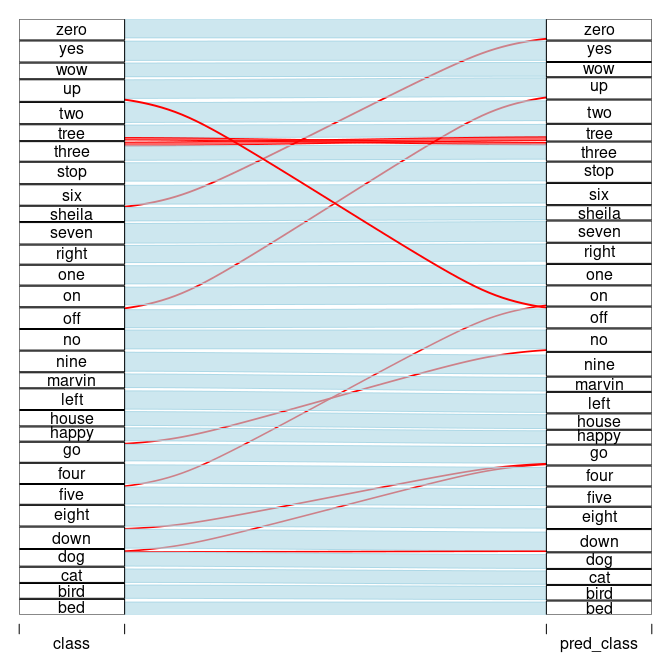
Model performance: true labels <--> predicted labels.

(#fig:unnamed-chunk-15)Model performance: true labels <–> predicted labels.

Model accuracy is 87,7%, somewhat worse than tensorflow version from the original post. Nevertheless, all conclusions from original post still hold.

Categories
Offsites

Simple audio classification with torch

This article translates Daniel Falbel’s ‘Simple Audio Classification’ article from tensorflow/keras to torch/torchaudio. The main goal is to introduce torchaudio and illustrate its contributions to the torch ecosystem. Here, we focus on a popular dataset, the audio loader and the spectrogram transformer. An interesting side product is the parallel between torch and tensorflow, showing sometimes the differences, sometimes the similarities between them.

library(torch)
library(torchaudio)

Downloading and Importing

torchaudio has the speechcommand_dataset built in. It filters out background_noise by default and lets us choose between versions v0.01 and v0.02.

# set an existing folder here to cache the dataset
DATASETS_PATH <- "~/datasets/"

# 1.4GB download
df <- speechcommand_dataset(
  root = DATASETS_PATH, 
  url = "speech_commands_v0.01",
  download = TRUE
)

# expect folder: _background_noise_
df$EXCEPT_FOLDER
# [1] "_background_noise_"

# number of audio files
length(df)
# [1] 64721

# a sample
sample <- df[1]

sample$waveform[, 1:10]
torch_tensor
0.0001 *
 0.9155  0.3052  1.8311  1.8311 -0.3052  0.3052  2.4414  0.9155 -0.9155 -0.6104
[ CPUFloatType{1,10} ]
sample$sample_rate
# 16000
sample$label
# bed

plot(sample$waveform[1], type = "l", col = "royalblue", main = sample$label)
A sample waveform for a 'bed'.

(#fig:unnamed-chunk-4)A sample waveform for a ‘bed’.

Classes

df$classes
 [1] "bed"    "bird"   "cat"    "dog"    "down"   "eight"  "five"  
 [8] "four"   "go"     "happy"  "house"  "left"   "marvin" "nine"  
[15] "no"     "off"    "on"     "one"    "right"  "seven"  "sheila"
[22] "six"    "stop"   "three"  "tree"   "two"    "up"     "wow"   
[29] "yes"    "zero"  

Generator Dataloader

torch::dataloader has the same task as data_generator defined in the original article. It is responsible for preparing batches – including shuffling, padding, one-hot encoding, etc. – and for taking care of parallelism / device I/O orchestration.

In torch we do this by passing the train/test subset to torch::dataloader and encapsulating all the batch setup logic inside a collate_fn() function.

set.seed(6)
id_train <- sample(length(df), size = 0.7*length(df))
id_test <- setdiff(seq_len(length(df)), id_train)
# subsets

train_subset <- torch::dataset_subset(df, id_train)
test_subset <- torch::dataset_subset(df, id_test)

At this point, dataloader(train_subset) would not work because the samples are not padded. So we need to build our own collate_fn() with the padding strategy.

I suggest using the following approach when implementing the collate_fn():

  1. begin with collate_fn <- function(batch) browser().
  2. instantiate dataloader with the collate_fn()
  3. create an environment by calling enumerate(dataloader) so you can ask to retrieve a batch from dataloader.
  4. run environment[[1]][[1]]. Now you should be sent inside collate_fn() with access to batch input object.
  5. build the logic.
collate_fn <- function(batch) {
  browser()
}

ds_train <- dataloader(
  train_subset, 
  batch_size = 32, 
  shuffle = TRUE, 
  collate_fn = collate_fn
)

ds_train_env <- enumerate(ds_train)
ds_train_env[[1]][[1]]

The final collate_fn() pads the waveform to length 16001 and then stacks everything up together. At this point there are no spectrograms yet. We going to make spectrogram transformation a part of model architecture.

pad_sequence <- function(batch) {
    # Make all tensors in a batch the same length by padding with zeros
    batch <- sapply(batch, function(x) (x$t()))
    batch <- torch::nn_utils_rnn_pad_sequence(batch, batch_first = TRUE, padding_value = 0.)
    return(batch$permute(c(1, 3, 2)))
  }

# Final collate_fn
collate_fn <- function(batch) {
 # Input structure:
 # list of 32 lists: list(waveform, sample_rate, label, speaker_id, utterance_number)
 # Transpose it
 batch <- purrr::transpose(batch)
 tensors <- batch$waveform
 targets <- batch$label_index

 # Group the list of tensors into a batched tensor
 tensors <- pad_sequence(tensors)
 
 # target encoding
 targets <- torch::torch_stack(targets)

 list(tensors = tensors, targets = targets) # (64, 1, 16001)
}

Batch structure is:

  • batch[[1]]: waveforms – tensor with dimension (32, 1, 16001)
  • batch[[2]]: targets – tensor with dimension (32, 1)

Also, torchaudio comes with 3 loaders, av_loader, tuner_loader, and audiofile_loader- more to come. set_audio_backend() is used to set one of them as the audio loader. Their performances differ based on audio format (mp3 or wav). There is no perfect world yet: tuner_loader is best for mp3, audiofile_loader is best for wav, but neither of them has the option of partially loading a sample from an audio file without bringing all the data into memory first.

For a given audio backend we need pass it to each worker through worker_init_fn() argument.

ds_train <- dataloader(
  train_subset, 
  batch_size = 128, 
  shuffle = TRUE, 
  collate_fn = collate_fn,
  num_workers = 16,
  worker_init_fn = function(.) {torchaudio::set_audio_backend("audiofile_loader")},
  worker_globals = c("pad_sequence") # pad_sequence is needed for collect_fn
)

ds_test <- dataloader(
  test_subset, 
  batch_size = 64, 
  shuffle = FALSE, 
  collate_fn = collate_fn,
  num_workers = 8,
  worker_globals = c("pad_sequence") # pad_sequence is needed for collect_fn
)

Model definition

Instead of keras::keras_model_sequential(), we are going to define a torch::nn_module(). As referenced by the original article, the model is based on this architecture for MNIST from this tutorial, and I’ll call it ‘DanielNN’.

dan_nn <- torch::nn_module(
  "DanielNN",
  
  initialize = function(
    window_size_ms = 30, 
    window_stride_ms = 10
  ) {
    
    # spectrogram spec
    window_size <- as.integer(16000*window_size_ms/1000)
    stride <- as.integer(16000*window_stride_ms/1000)
    fft_size <- as.integer(2^trunc(log(window_size, 2) + 1))
    n_chunks <- length(seq(0, 16000, stride))
    
    self$spectrogram <- torchaudio::transform_spectrogram(
      n_fft = fft_size, 
      win_length = window_size, 
      hop_length = stride, 
      normalized = TRUE, 
      power = 2
    )
    
    # convs 2D
    self$conv1 <- torch::nn_conv2d(in_channels = 1, out_channels = 32, kernel_size = c(3,3))
    self$conv2 <- torch::nn_conv2d(in_channels = 32, out_channels = 64, kernel_size = c(3,3))
    self$conv3 <- torch::nn_conv2d(in_channels = 64, out_channels = 128, kernel_size = c(3,3))
    self$conv4 <- torch::nn_conv2d(in_channels = 128, out_channels = 256, kernel_size = c(3,3))
    
    # denses
    self$dense1 <- torch::nn_linear(in_features = 14336, out_features = 128)
    self$dense2 <- torch::nn_linear(in_features = 128, out_features = 30)
  },
  
  forward = function(x) {
    x %>% # (64, 1, 16001)
      self$spectrogram() %>% # (64, 1, 257, 101)
      torch::torch_add(0.01) %>%
      torch::torch_log() %>%
      self$conv1() %>%
      torch::nnf_relu() %>%
      torch::nnf_max_pool2d(kernel_size = c(2,2)) %>%
      
      self$conv2() %>%
      torch::nnf_relu() %>%
      torch::nnf_max_pool2d(kernel_size = c(2,2)) %>%
      
      self$conv3() %>%
      torch::nnf_relu() %>%
      torch::nnf_max_pool2d(kernel_size = c(2,2)) %>%
      
      self$conv4() %>%
      torch::nnf_relu() %>%
      torch::nnf_max_pool2d(kernel_size = c(2,2)) %>%
      
      torch::nnf_dropout(p = 0.25) %>%
      torch::torch_flatten(start_dim = 2) %>%
      
      self$dense1() %>%
      torch::nnf_relu() %>%
      torch::nnf_dropout(p = 0.5) %>%
      self$dense2() 
  }
)

model <- dan_nn()


device <- torch::torch_device(if(torch::cuda_is_available()) "cuda" else "cpu")
model$to(device = device)

print(model)
An `nn_module` containing 2,226,846 parameters.

── Modules ──────────────────────────────────────────────────────
● spectrogram: <Spectrogram> #0 parameters
● conv1: <nn_conv2d> #320 parameters
● conv2: <nn_conv2d> #18,496 parameters
● conv3: <nn_conv2d> #73,856 parameters
● conv4: <nn_conv2d> #295,168 parameters
● dense1: <nn_linear> #1,835,136 parameters
● dense2: <nn_linear> #3,870 parameters

Model fitting

Unlike in tensorflow, there is no model %>% compile(…) step in torch, so we are going to set loss criterion, optimizer strategy and evaluation metrics explicitly in the training loop.

loss_criterion <- torch::nn_cross_entropy_loss()
optimizer <- torch::optim_adadelta(model$parameters, rho = 0.95, eps = 1e-7)
metrics <- list(acc = yardstick::accuracy_vec)

Training loop

library(glue)
library(progress)

pred_to_r <- function(x) {
  classes <- factor(df$classes)
  classes[as.numeric(x$to(device = "cpu"))]
}

set_progress_bar <- function(total) {
  progress_bar$new(
    total = total, clear = FALSE, width = 70,
    format = ":current/:total [:bar] - :elapsed - loss: :loss - acc: :acc"
  )
}
epochs <- 20
losses <- c()
accs <- c()

for(epoch in seq_len(epochs)) {
  pb <- set_progress_bar(length(ds_train))
  pb$message(glue("Epoch {epoch}/{epochs}"))
  coro::loop(for(batch in ds_train) {
    optimizer$zero_grad()
    predictions <- model(batch[[1]]$to(device = device))
    targets <- batch[[2]]$to(device = device)
    loss <- loss_criterion(predictions, targets)
    loss$backward()
    optimizer$step()
    
    # eval reports
    prediction_r <- pred_to_r(predictions$argmax(dim = 2))
    targets_r <- pred_to_r(targets)
    acc <- metrics$acc(targets_r, prediction_r)
    accs <- c(accs, acc)
    loss_r <- as.numeric(loss$item())
    losses <- c(losses, loss_r)
    
    pb$tick(tokens = list(loss = round(mean(losses), 4), acc = round(mean(accs), 4)))
  })
}


# test
predictions_r <- c()
targets_r <- c()
coro::loop(for(batch_test in ds_test) {
  predictions <- model(batch_test[[1]]$to(device = device))
  targets <- batch_test[[2]]$to(device = device)
  predictions_r <- c(predictions_r, pred_to_r(predictions$argmax(dim = 2)))
  targets_r <- c(targets_r, pred_to_r(targets))
})
val_acc <- metrics$acc(factor(targets_r, levels = 1:30), factor(predictions_r, levels = 1:30))
cat(glue("val_acc: {val_acc}nn"))
Epoch 1/20                                                            
[W SpectralOps.cpp:590] Warning: The function torch.rfft is deprecated and will be removed in a future PyTorch release. Use the new torch.fft module functions, instead, by importing torch.fft and calling torch.fft.fft or torch.fft.rfft. (function operator())
354/354 [=========================] -  1m - loss: 2.6102 - acc: 0.2333
Epoch 2/20                                                            
354/354 [=========================] -  1m - loss: 1.9779 - acc: 0.4138
Epoch 3/20                                                            
354/354 [============================] -  1m - loss: 1.62 - acc: 0.519
Epoch 4/20                                                            
354/354 [=========================] -  1m - loss: 1.3926 - acc: 0.5859
Epoch 5/20                                                            
354/354 [==========================] -  1m - loss: 1.2334 - acc: 0.633
Epoch 6/20                                                            
354/354 [=========================] -  1m - loss: 1.1135 - acc: 0.6685
Epoch 7/20                                                            
354/354 [=========================] -  1m - loss: 1.0199 - acc: 0.6961
Epoch 8/20                                                            
354/354 [=========================] -  1m - loss: 0.9444 - acc: 0.7181
Epoch 9/20                                                            
354/354 [=========================] -  1m - loss: 0.8816 - acc: 0.7365
Epoch 10/20                                                           
354/354 [=========================] -  1m - loss: 0.8278 - acc: 0.7524
Epoch 11/20                                                           
354/354 [=========================] -  1m - loss: 0.7818 - acc: 0.7659
Epoch 12/20                                                           
354/354 [=========================] -  1m - loss: 0.7413 - acc: 0.7778
Epoch 13/20                                                           
354/354 [=========================] -  1m - loss: 0.7064 - acc: 0.7881
Epoch 14/20                                                           
354/354 [=========================] -  1m - loss: 0.6751 - acc: 0.7974
Epoch 15/20                                                           
354/354 [=========================] -  1m - loss: 0.6469 - acc: 0.8058
Epoch 16/20                                                           
354/354 [=========================] -  1m - loss: 0.6216 - acc: 0.8133
Epoch 17/20                                                           
354/354 [=========================] -  1m - loss: 0.5985 - acc: 0.8202
Epoch 18/20                                                           
354/354 [=========================] -  1m - loss: 0.5774 - acc: 0.8263
Epoch 19/20                                                           
354/354 [==========================] -  1m - loss: 0.5582 - acc: 0.832
Epoch 20/20                                                           
354/354 [=========================] -  1m - loss: 0.5403 - acc: 0.8374
val_acc: 0.876705979296493

Making predictions

We already have all predictions calculated for test_subset, let’s recreate the alluvial plot from the original article.

library(dplyr)
library(alluvial)
df_validation <- data.frame(
  pred_class = df$classes[predictions_r],
  class = df$classes[targets_r]
)
x <-  df_validation %>%
  mutate(correct = pred_class == class) %>%
  count(pred_class, class, correct)

alluvial(
  x %>% select(class, pred_class),
  freq = x$n,
  col = ifelse(x$correct, "lightblue", "red"),
  border = ifelse(x$correct, "lightblue", "red"),
  alpha = 0.6,
  hide = x$n < 20
)
Model performance: true labels <--> predicted labels.

(#fig:unnamed-chunk-15)Model performance: true labels <–> predicted labels.

Model accuracy is 87,7%, somewhat worse than tensorflow version from the original post. Nevertheless, all conclusions from original post still hold.

Categories
Misc

Latest from google researchers: state of the art in video stabilization!

Latest from google researchers: state of the art in video stabilization! submitted by /u/MLtinkerer
[visit reddit] [comments]
Categories
Misc

Latest from KDnuggets: Find code implementation for any AI/ML paper using this new chrome extension

submitted by /u/MLtinkerer
[visit reddit] [comments]

Categories
Misc

Training architecture fro scratch to use with the object detection API

For my thesis, I am attempting to detect faults/inconsistencies in 3D prints.
Generating data takes a long time (because the print process takes a long time). For this reason my dataset is limited. I’ve got two classes which each have about 100-150 images each. This adds up to a total of about 250-300 images.Then I augmented those images 8 times with rotations and flips. I first tried to train on EfficientdetD0 but the results were pretty disappointing. Perhaps only a quarter of errors were getting detected.
Someone on this subreddit told me I should use an architecture like ” SSD ResNet50 V1 FPN 640×640 (RetinaNet50) ” because this appearantly works better for small datasets, though I don’t know why. So I went and tried it. I trained with the same parameters as before and for roughly the same time. The results were even worse.

Right now I would like to train a model from scratch and compare the results to the results I got using transfer learning, however I have no clue on how I should get started with this. I’ve been googling about but I haven’t found a clear explanation just yet. Could somebody please point me in the right direction?

Also why should SSD ResNet50 V1 FPN 640×640 (RetinaNet50) work better with smaller datasets, and why shouldn’t I just use ResNet 151? From what I’ve gathered this should work better than 50 in my case because it goed deeper, no?

submitted by /u/007Nick700
[visit reddit] [comments]