Categories
Offsites

Bayes Theorem, maximum likelihood estimation and TensorFlow Probability

A growing trend in deep learning (and machine learning in general) is a probabilistic or Bayesian approach to the problem. Why is this? Simply put – a standard deep learning model produces a prediction, but with no statistically robust understanding of how confident the model is in the prediction. This is important in the understanding of the limitations of model predictions, and also if one wants to do probabilistic modeling of any kind. There are also other applications, such as probabilistic programming and being able to use domain knowledge, but more on that in another post. The TensorFlow developers have addressed this problem by creating TensorFlow Probability. This post will introduce some basic Bayesian concepts, specifically the likelihood function and maximum likelihood estimation, and how these can be used in TensorFlow Probability for the modeling of a simple function.

The code contained in this tutorial can be found on this site’s Github repository.


Eager to build deep learning systems in TensorFlow 2? Get the book here


Bayes theorem and maximum likelihood estimation

Bayes theorem is one of the most important statistical concepts a machine learning practitioner or data scientist needs to know. In the machine learning context, it can be used to estimate the model parameters (e.g. the weights in a neural network) in a statistically robust way. It can also be used in model selection e.g. choosing which machine learning model is the best to address a given problem. I won’t be going in-depth into all the possible uses of Bayes theorem here, however, but I will be introducing the main components of the theorem.

Bayes theorem can be shown in a fairly simple equation involving conditional probabilities as follows:

$$P(theta vert D) = frac{P(D vert theta) P(theta)}{P(D)}$$

In this representation, the variable $theta$ corresponds to the model parameters (i.e. the values of the weights in a neural network), and the variable $D$ corresponds to the data that we are using to estimate the $theta$ values. Before I talk about what conditional probabilities are, I’ll just quickly point out three terms in this formula which are very important to familiarise yourself with, as they come up in the literature all the time. It is worthwhile memorizing what these terms refer to:

$P(theta vert D)$ – this is called the posterior

$P(D vert theta)$ – this is called the likelihood

$P(theta)$ – this is called the prior

I’m going to explain what all these terms refer to shortly, but first I’ll make a quick detour to discuss conditional probability for those who may not be familiar. If you are already familiar with conditional probability, feel free to skip this section.

Conditional probability

Conditional probability is an important statistical concept that is thankfully easy to understand, as it forms a part of our everyday reasoning. Let’s say we have a random variable called RT which represents whether it will rain today – it is a discrete variable and can take on the value of either 1 or 0, denoting whether it will rain today or not. Let’s say we are in a fairly dry environment, and by consulting some long-term rainfall records we know that RT=1 about 10% of the time, and therefore RT=0 about 90% of the time. This fully represents the probability function for RT which can be written as P(RT). Therefore, we have some prior knowledge of what P(RT) is in the absence of any other determining factors.

Ok, so what does P(RT) look like if we know it rained yesterday? Is it the same or is it different? Well, let’s say the region we are in gets most of its rainfall due to big weather systems that can last for days or weeks – in this case, we have good reason to believe that P(RT) will be different given the fact that it rained yesterday. Therefore, the probability P(RT) is now conditioned on our understanding of another random variable P(RY) which represents whether it has rained yesterday. The way of showing this conditional probability is by using the vertical slash symbol $vert$ – so the conditional probability that it will rain today given it rained yesterday looks like the following: $P(RT=1 vert RY = 1)$. Perhaps for this reason the probability that it will rain today is no longer 10%, but maybe will rise to 30%, so $P(RT=1 vert RY = 1) = 0.3$

We could also look at other probabilities, such as $P(RT=1 vert RY = 0)$ or $P(RT=0 vert RY = 1)$ and so on. To generalize this relationship we would just write $P(RT vert RY)$.

Now that you have an understanding of conditional probabilities, let’s move on to explaining Bayes Theorem (which contains two conditional probability functions) in more detail.

Bayes theorem in more detail

The posterior

Ok, so as I stated above, it is time to delve into the meaning of the individual terms of Bayes theorem. Let’s first look at the posterior term – $P(theta vert D)$. This term can be read as: given we have a certain dataset $D$, what is the probability of our parameters $theta$? This is the term we want to maximize when varying the parameters of a model according to a dataset – by doing so, we find those parameters $theta$ which are most probable given the model we are using and the training data supplied. The posterior is on the left-hand side of the equation of Bayes Theorem, so if we want to maximize the posterior we can do this by maximizing the right-hand side of the equation.

Let’s have a look at the terms on the right-hand side.

The likelihood

The likelihood is expressed as $P(D vert theta)$ and can be read as: given this parameter $theta$, which defines some process of generating data, what is the probability we would see this given set of data $D$? Let’s say we have a scattering of data-points – a good example might be the heights of all the members of a classroom full of kids. We can define a model that we assume is able to generate or represent this data – in this case, the Normal distribution is a good choice. The parameters that we are trying to determine in the Normal distribution is the tuple ($mu$, $sigma$) – the mean and variance of the Normal distribution.

So the likelihood $P(D vert theta)$ in this example is the probability of seeing this sample of measured heights given different values of the mean and variance of the Normal distribution function. There is some more mathematical precision needed here (such as the difference between a probability distribution and a probability density function, discrete samples etc.) but this is ok for our purposes of coming to a conceptual understanding.

I’ll come back to the concept of the likelihood shortly when we discuss maximum likelihood estimation, but for now, let’s move onto the prior.

The prior

The prior probability $P(theta)$, as can be observed, is not a conditioned probability distribution. It is simply a representation of the probability of the parameters prior to any other consideration of data or evidence. You may be puzzled as to what the point of this probability is. In the context of machine learning or probabilistic programming, it’s purpose is to enable us to specify some prior understanding of what the parameters should actually be, and the prior probability distribution it should be drawn from.

Returning to the example of the heights of kids in a classroom. Let’s say the teacher is a pretty good judge of heights, and therefore he or she can come to the problem with a rough prior estimate of what the mean height would be. Let’s say he or she guesses that the average height is around 130cm. He can then put a prior around the mean parameter $mu$ of, say, a normal distribution with a mean of 130cm.

The presence of the prior in the Bayes theorem allows us to introduce expert knowledge or prior beliefs into the problem, which aids the finding of the optimal parameters $theta$. These prior beliefs are then updated by the data collected $D$ – with the updating occurring through the action of the likelihood function.

The graph below is an example of the evolution of a prior distribution function exposed to some set of data:

The evolution of the prior - Bayes Theorem - Maximum likelihood estimation

The evolution of the prior distribution towards the evidence / data

Here we can see that, through the application of the Bayes Theorem, we can start out with a certain set of prior beliefs in the form of a prior distribution function, but by applying the evidence or data through the likelihood $P(D vert theta)$, the posterior estimate $P(theta vert D)$ moves closer to “reality”.

The data

The final term in Bayes Theorem is the unconditioned probability distribution of the process that generated the data $P(D)$. In machine learning applications, this distribution is often unknown – but thankfully, it doesn’t matter. This distribution acts as a normalization constant and has nothing to say about the parameters we are trying to estimate $theta$. Therefore, because we are trying to simply maximize the right-hand side of the equation, it drops out of any derivative calculation that is made in order to find the maximum. So in the context of machine learning and estimating parameters, this term can be safely ignored. Given this understanding, the form of Bayes Theorem that we are mostly interested in for machine learning purposes is as follows: $$P(theta vert D) propto P(D vert theta) P(theta)$$

Given this formulation, all we are concerned about is either maximizing the right-hand side of the equation or by simulating the sampling of the posterior itself (not covered in this post).

How to estimate the posterior

Now that we have reviewed conditional probability concepts and Bayes Theorem, it is now time to consider how to apply Bayes Theorem in practice to estimate the best parameters in a machine learning problem. There are a number of ways of estimating the posterior of the parameters in a machine learning problem. These include maximum likelihood estimation, maximum a posterior probability (MAP) estimation, simulating the sampling from the posterior using Markov Chain Monte Carlo (MCMC) methods such as Gibbs sampling, and so on. In this post, I will just be considering maximum likelihood estimation (MLE) with other methods being considered in future content on this site.

Maximum likelihood estimation (MLE)

What happens if we just throw our hands up in the air with regards to the prior $P(theta)$ and say we don’t know anything about the best parameters to describe the data? In that case, the prior becomes a uniform or un-informative prior – in that case, $P(theta)$ becomes a constant (same probability no matter what the parameter values are), and our Bayes Theorem reduces to:

$$P(theta vert D) propto P(D vert theta)$$

If this is the case, all we have to do is maximize the likelihood $P(D vert theta)$ and by doing so we will also find the maximum of the posterior – i.e. the parameter with the highest probability given our model and data – or, in short, an estimate of the optimal parameters. If we have a way of calculating $P(D vert theta)$ while varying the parameters $theta$, we can then feed this into some sort of optimizer to calculate:

$$underset{theta}{operatorname{argmax}} P(D vert theta)$$
 
Nearly always, instead of maximizing $P(D vert theta)$ the log of $P(D vert theta)$ is maximized. Why? If we were doing the calculations by hand, we would need to calculate the derivative of the product of multiple exponential functions (as probability functions like the Normal distribution have exponentials in them) which is tricky. Because logs are monotonically increasing functions, they have maximums at the same point as the non-log function. So in other words, the maximum likelihood will occur at the same parameter value as the maximum of the log likelihood. By taking the log of the likelihood, products turn into sums and this makes derivative calculations a whole lot easier.
 
Finally, some optimizers in machine learning packages such as TensorFlow only minimize loss functions, so we need to invert the sign of the loss function in order to maximize it. In that case, for maximum likelihood estimation, we would minimize the negative log likelihood, or NLL, and get the same result.
 
Let’s look at a simple example of maximum likelihood estimation by using TensorFlow Probability.

TensorFlow Probability and maximum likelihood estimation

For the simple example of maximum likelihood estimation that is to follow, TensorFlow Probability is overkill – however, TensorFlow Probability is a great extension of TensorFlow into the statistical domain, so it is worthwhile introducing MLE by utilizing it. The Jupyter Notebook containing this example can be found at this site’s Github repository. Note this example is loosely based on the TensorFlow tutorial found here. In this example, we will be estimating linear regression parameters based on noisy data. These parameters can obviously be solved using analytical techniques, but that isn’t as interesting. First, we import some libraries and generate the noisy data:

import tensorflow as tf
import tensorflow_probability as tfp
import numpy as np
import matplotlib.pylab as plt
tfd = tfp.distributions

x_range = np.arange(0, 10, 0.1)
grad = 2.0
intercept = 3.0
lin_reg = x_range * grad + np.random.normal(0, 3.0, len(x_range)) + intercept

Plotting our noisy regression line looks like the following:

Noisy regression line - Maximum likelihood estimation

Noisy regression line

Next, let’s set up our little model to predict the underlying regression function from the noisy data:

model = tf.keras.Sequential([
  tf.keras.layers.Dense(1),
  tfp.layers.DistributionLambda(lambda x: tfd.Normal(loc=x, scale=1)),
])

So here we have a simple Keras sequential model (for more detail on Keras and TensorFlow, see this post). The first layer is a Dense layer with one node. Given each Dense layer has one bias input by default – this layer equates to generating a simple line with a gradient and intercept: $xW + b$ where x is the input data, W is the single input weight and b is the bias weight. So the first Dense layer produces a line with a trainable gradient and y-intercept value.

The next layer is where TensorFlow Probability comes in. This layer allows you to create a parameterized probability distribution, with the parameter being “fed in” from the output of previous layers. In this case, you can observe that the lambda x, which is the output from the previous layer, is defining the mean of a Normal distribution. In this case, the scale (i.e. the standard deviation) is fixed to 1.0. So, using TensorFlow probability, our model no longer will just predict a single value for each input (as in a non-probabilistic neural network) – no, instead the output is actually a Normal distribution. In that case, to actually predict values we need to call statistical functions from the output of the model. For instance:

  • model(np.array([[1.0]])).sample(10) will produce a random sample of 10 outputs from the Normal distribution, parameterized by the input value 1.0 fed through the first Dense layer
  • model(np.array([[1.0]])).mean() will produce the mean of the distribution, given the input
  • model(np.array([[1.0]])).stddev() will produce the standard deviation of the distribution, given the input

and so on. We can also calculate the log probability of the output distribution, as will be discussed shortly. Next, we need to set up our “loss” function – in this case, our “loss” function is actually just the negative log likelihood (NLL):

def neg_log_likelihood(y_actual, y_predict):
  return -y_predict.log_prob(y_actual)

In the above, the y_actual values are the actual noisy training samples. The values y_predict are actually a tensor of parameterized Normal probability distributions – one for each different training input. So, for instance, if one training input is 5.0, the corresponding y_predict value will be a Normal distribution with a mean value of, say, 12. Another training input may have a value 10.0, and the corresponding y_predict will be a Normal distribution with a mean value of, say, 20, and so on. Therefore, for each y_predict and y_actual pair, it is possible to calculate the log probability of that actual value occurring given the predicted Normal distribution.

To make this more concrete – let’s say for a training input value 5.0, the corresponding actual noisy regression value is 8.0. However, let’s say the predicted Normal distribution has a mean of 10.0 (and a fixed variance of 1.0). Using the formula for the log probability / log likelihood of a Normal distribution:

$$ell_x(mu,sigma^2) = – ln sigma – frac{1}{2} ln (2 pi) – frac{1}{2} Big( frac{x-mu}{sigma} Big)^2$$

Substituting in the example values mentioned above:

$$ell_x(10.0,1.0) = – ln 1.0 – frac{1}{2} ln (2 pi) – frac{1}{2} Big( frac{8.0-10.0}{1.0} Big)^2$$

We can calculate the log likelihood from the y_predict distribution and the y_actual values. Of course, TensorFlow Probability does this for us by calling the log_prob method on the y_predict distribution. Taking the negative of this calculation, as I have done in the function above, gives us the negative log likelihood value that we need to minimize to perform MLE.

After the loss function, it is now time to compile the model, train it, and make some predictions:

model.compile(optimizer=tf.optimizers.Adam(learning_rate=0.05), loss=neg_log_likelihood)
model.fit(x_range, lin_reg, epochs=500, verbose=False)

yhat = model(x_range)
mean = yhat.mean()

As can be observed, the model is compiled using our custom neg_log_likelihood function as the loss. Because this is just a toy example, I am using the full dataset as both the train and test set. The estimated regression line is simply the mean of all the predicted distributions, and plotting it produces the following:

plt.close("all")
plt.scatter(x_range, lin_reg)
plt.plot(x_range, mean, label='predicted')
plt.plot(x_range, x_range * grad + intercept, label='ground truth')
plt.legend(loc="upper left")
plt.show()
plt.close("all") plt.scatter(x_range, lin_reg) plt.plot(x_range, mean, label='predicted') plt.plot(x_range, x_range * grad + intercept, label='ground truth') plt.legend(loc="upper left") plt.show()

TensorFlow Probability based regression using maximum likelihood estimation

Another example with changing variance

Another, more interesting, example is to use the model to predict not only the mean but also the changing variance of a dataset. In this example, the dataset consists of the same trend but the noise variance increases along with the values:

def noise(x, grad=0.5, const=2.0):
  return np.random.normal(0, grad * x + const)

x_range = np.arange(0, 10, 0.1)
noise = np.array(list(map(noise, x_range)))
grad = 2.0
intercept = 3.0
lin_reg = x_range * grad + intercept + noise

plt.scatter(x_range, lin_reg)
plt.show()
linear regression with increasing noise variance

Linear regression with increasing noise variance

The new model looks like the following:

model = tf.keras.Sequential([
  tf.keras.layers.Dense(2),
  tfp.layers.DistributionLambda(lambda x: tfd.Normal(loc=x[:, 0], scale=1e-3 + tf.math.softplus(0.3 * x[:, 1]))),
])

In this case, we have two nodes in the first layer, ostensibly to predict both the mean and standard deviation of the Normal distribution, instead of just the mean as in the last example. The mean of the distribution is assigned to the output of the first node (x[:, 0]) and the standard deviation / scale is set to be equal to a softplus function based on the output of the second node (x[:, 1]). After training this model on the same data and using the same loss as the previous example, we can predict both the mean and standard deviation of the model like so:

mean = yhat.mean()
upper = mean + 2 * yhat.stddev()
lower = mean - 2 * yhat.stddev()

In this case, the upper and lower variables are the 2-standard deviation upper and lower bounds of the predicted distributions. Plotting this produces:

plt.close("all")
plt.scatter(x_range, lin_reg)
plt.plot(x_range, mean, label='predicted')
plt.fill_between(x_range, lower, upper, alpha=0.1)
plt.plot(x_range, x_range * grad + intercept, label='ground truth')
plt.legend(loc="upper left")
plt.show()
Regression prediction with increasing variance

Regression prediction with increasing variance

As can be observed, the model is successfully predicting the increasing variance of the dataset, along with the mean of the trend. This is a limited example of the power of TensorFlow Probability, but in future posts I plan to show how to develop more complicated applications like Bayesian Neural Networks. I hope this post has been useful for you in getting up to speed in topics such as conditional probability, Bayes Theorem, the prior, posterior and likelihood function, maximum likelihood estimation and a quick introduction to TensorFlow Probability. Look out for future posts expanding on the increasingly important probabilistic side of machine learning.


Eager to build deep learning systems in TensorFlow 2? Get the book here


The post Bayes Theorem, maximum likelihood estimation and TensorFlow Probability appeared first on Adventures in Machine Learning.

Categories
Offsites

Python TensorFlow Tutorial – Build a Neural Network

Updated for TensorFlow 2

Google’s TensorFlow has been a hot topic in deep learning recently.  The open source software, designed to allow efficient computation of data flow graphs, is especially suited to deep learning tasks.  It is designed to be executed on single or multiple CPUs and GPUs, making it a good option for complex deep learning tasks.  In its most recent incarnation – version 1.0 – it can even be run on certain mobile operating systems.  This introductory tutorial to TensorFlow will give an overview of some of the basic concepts of TensorFlow in Python.  These will be a good stepping stone to building more complex deep learning networks, such as Convolution Neural Networks, natural language models, and Recurrent Neural Networks in the package.  We’ll be creating a simple three-layer neural network to classify the MNIST dataset.  This tutorial assumes that you are familiar with the basics of neural networks, which you can get up to scratch with in the neural networks tutorial if required.  To install TensorFlow, follow the instructions here. The code for this tutorial can be found in this site’s GitHub repository.  Once you’re done, you also might want to check out a higher level deep learning library that sits on top of TensorFlow called Keras – see my Keras tutorial.

First, let’s have a look at the main ideas of TensorFlow.

1.0 TensorFlow graphs

TensorFlow is based on graph based computation – “what on earth is that?”, you might say.  It’s an alternative way of conceptualising mathematical calculations.  Consider the following expression $a = (b + c) * (c + 2)$.  We can break this function down into the following components:

begin{align}
d &= b + c \
e &= c + 2 \
a &= d * e
end{align}

Now we can represent these operations graphically as:

TensorFlow tutorial - simple computational graph

Simple computational graph

This may seem like a silly example – but notice a powerful idea in expressing the equation this way: two of the computations ($d=b+c$ and $e=c+2$) can be performed in parallel.  By splitting up these calculations across CPUs or GPUs, this can give us significant gains in computational times.  These gains are a must for big data applications and deep learning – especially for complicated neural network architectures such as Convolutional Neural Networks (CNNs) and Recurrent Neural Networks (RNNs).  The idea behind TensorFlow is to the ability to create these computational graphs in code and allow significant performance improvements via parallel operations and other efficiency gains.

We can look at a similar graph in TensorFlow below, which shows the computational graph of a three-layer neural network.

TensorFlow tutorial - data flow graph

TensorFlow data flow graph

The animated data flows between different nodes in the graph are tensors which are multi-dimensional data arrays.  For instance, the input data tensor may be 5000 x 64 x 1, which represents a 64 node input layer with 5000 training samples.  After the input layer, there is a hidden layer with rectified linear units as the activation function.  There is a final output layer (called a “logit layer” in the above graph) that uses cross-entropy as a cost/loss function.  At each point we see the relevant tensors flowing to the “Gradients” block which finally flows to the Stochastic Gradient Descent optimizer which performs the back-propagation and gradient descent.

Here we can see how computational graphs can be used to represent the calculations in neural networks, and this, of course, is what TensorFlow excels at.  Let’s see how to perform some basic mathematical operations in TensorFlow to get a feel for how it all works.

2.0 A Simple TensorFlow example

So how can we make TensorFlow perform the little example calculation shown above – $a = (b + c) * (c + 2)$? First, there is a need to introduce TensorFlow variables.  The code below shows how to declare these objects:

import tensorflow as tf
# create TensorFlow variables
const = tf.Variable(2.0, name="const")
b = tf.Variable(2.0, name='b')
c = tf.Variable(1.0, name='c')

As can be observed above, TensorFlow variables can be declared using the tf.Variable function.  The first argument is the value to be assigned to the variable. The second is an optional name string which can be used to label the constant/variable – this is handy for when you want to do visualizations.  TensorFlow will infer the type of the variable from the initialized value, but it can also be set explicitly using the optional dtype argument.  TensorFlow has many of its own types like tf.float32, tf.int32 etc.

The objects assigned to the Python variables are actually TensorFlow tensors. Thereafter, they act like normal Python objects – therefore, if you want to access the tensors you need to keep track of the Python variables. In previous versions of TensorFlow, there were global methods of accessing the tensors and operations based on their names. This is no longer the case.

To examine the tensors stored in the Python variables, simply call them as you would a normal Python variable. If we do this for the “const” variable, you will see the following output:

<tf.Variable ‘const:0′ shape=() dtype=float32, numpy=2.0>

This output gives you a few different pieces of information – first, is the name ‘const:0’ which has been assigned to the tensor. Next is the data type, in this case, a TensorFlow float 32 type. Finally, there is a “numpy” value. TensorFlow variables in TensorFlow 2 can be converted easily into numpy objects. Numpy stands for Numerical Python and is a crucial library for Python data science and machine learning. If you don’t know Numpy, what it is, and how to use it, check out this site. The command to access the numpy form of the tensor is simply .numpy() – the use of this method will be shown shortly.

Next, some calculation operations are created:

# now create some operations
d = tf.add(b, c, name='d')
e = tf.add(c, const, name='e')
a = tf.multiply(d, e, name='a')

Note that d and e are automatically converted to tensor values upon the execution of the operations. TensorFlow has a wealth of calculation operations available to perform all sorts of interactions between tensors, as you will discover as you progress through this book.  The purpose of the operations shown above are pretty obvious, and they instantiate the operations b + c, c + 2.0, and d * e. However, these operations are an unwieldy way of doing things in TensorFlow 2. The operations below are equivalent to those above:

d = b + c
e = c + 2
a = d * e

To access the value of variable a, one can use the .numpy() method as shown below:

print(f”Variable a is {a.numpy()}”)

The computational graph for this simple example can be visualized by using the TensorBoard functionality that comes packaged with TensorFlow. This is a great visualization feature and is explained more in this post. Here is what the graph looks like in TensorBoard:

TensorFlow tutorial - simple graph

Simple TensorFlow graph

The larger two vertices or nodes, b and c, correspond to the variables. The smaller nodes correspond to the operations, and the edges between the vertices are the scalar values emerging from the variables and operations.

The example above is a trivial example – what would this look like if there was an array of b values from which an array of equivalent a values would be calculated? TensorFlow variables can easily be instantiated using numpy variables, like the following:

b = tf.Variable(np.arange(0, 10), name='b')

Calling b shows the following:

<tf.Variable ‘b:0′ shape=(10,) dtype=int32, numpy=array([0, 1, 2, 3, 4, 5, 6, 7, 8, 9])>

Note the numpy value of the tensor is an array. Because the numpy variable passed during the instantiation is a range of int32 values, we can’t add it directly to c as c is of float32 type. Therefore, the tf.cast operation, which changes the type of a tensor, first needs to be utilized like so:

d = tf.cast(b, tf.float32) + c

Running the rest of the previous operations, using the new b tensor, gives the following value for a:

Variable a is [ 3.  6.  9. 12. 15. 18. 21. 24. 27. 30.]

In numpy, the developer can directly access slices or individual indices of an array and change their values directly. Can the same be done in TensorFlow 2? Can individual indices and/or slices be accessed and changed? The answer is yes, but not quite as straight-forwardly as in numpy. For instance, if b was a simple numpy array, one could easily execute the following b[1] = 10 – this would change the value of the second element in the array to the integer 10.

b[1].assign(10)

This will then flow through to a like so:

Variable a is [ 3. 33.  9. 12. 15. 18. 21. 24. 27. 30.]

The developer could also run the following, to assign a slice of b values:

b[6:9].assign([10, 10, 10])

A new tensor can also be created by using the slice notation:

f = b[2:5]

The explanations and code above show you how to perform some basic tensor manipulations and operations. In the section below, an example will be presented where a neural network is created using the Eager paradigm in TensorFlow 2. It will show how to create a training loop, perform a feed-forward pass through a neural network and calculate and apply gradients to an optimization method.

3.0 A Neural Network Example

In this section, a simple three-layer neural network build in TensorFlow is demonstrated.  In following chapters more complicated neural network structures such as convolution neural networks and recurrent neural networks are covered.  For this example, though, it will be kept simple.

In this example, the MNIST dataset will be used that is packaged as part of the TensorFlow installation. This MNIST dataset is a set of 28×28 pixel grayscale images which represent hand-written digits.  It has 60,000 training rows, 10,000 testing rows, and 5,000 validation rows. It is a very common, basic, image classification dataset that is used in machine learning.

The data can be loaded by running the following:

from tensorflow.keras.datasets import mnist
(x_train, y_train), (x_test, y_test) = mnist.load_data()

As can be observed, the Keras MNIST data loader returns Python tuples corresponding to the training and test set respectively (Keras is another deep learning framework, now tightly integrated with TensorFlow, as mentioned earlier). The data sizes of the tuples defined above are:

  • x_train: (60,000 x 28 x 28)
  • y_train: (60,000)
  • x_test: (10,000 x 28 x 28)
  • y_test: (10,000)

The x data is the image information – 60,000 images of 28 x 28 pixels size in the training set. The images are grayscale (i.e black and white) with maximum values, specifying the intensity of whites, of 255. The x data will need to be scaled so that it resides between 0 and 1, as this improves training efficiency. The y data is the matching image labels – signifying what digit is displayed in the image. This will need to be transformed to “one-hot” format.

When using a standard, categorical cross-entropy loss function (this will be shown later), a one-hot format is required when training classification tasks, as the output layer of the neural network will have the same number of nodes as the total number of possible classification labels. The output node with the highest value is considered as a prediction for that corresponding label. For instance, in the MNIST task, there are 10 possible classification labels – 0 to 9. Therefore, there will be 10 output nodes in any neural network performing this classification task. If we have an example output vector of [0.01, 0.8, 0.25, 0.05, 0.10, 0.27, 0.55, 0.32, 0.11, 0.09], the maximum value is in the second position / output node, and therefore this corresponds to the digit “1”. To train the network to produce this sort of outcome when the digit “1” appears, the loss needs to be calculated according to the difference between the output of the network and a “one-hot” array of the label 1. This one-hot array looks like [0, 1, 0, 0, 0, 0, 0, 0, 0, 0].

This conversion is easily performed in TensorFlow, as will be demonstrated shortly when the main training loop is covered.

One final thing that needs to be considered is how to extract the training data in batches of samples. The function below can handle this:

def get_batch(x_data, y_data, batch_size):
    idxs = np.random.randint(0, len(y_data), batch_size)
    return x_data[idxs,:,:], y_data[idxs]

As can be observed in the code above, the data to be batched i.e. the x and y data is passed to this function along with the batch size. The first line of the function generates a random vector of integers, with random values between 0 and the length of the data passed to the function. The number of random integers generated is equal to the batch size. The x and y data are then returned, but the return data is only for those random indices chosen. Note, that this is performed on numpy array objects – as will be shown shortly, the conversion from numpy arrays to tensor objects will be performed “on the fly” within the training loop.

There is also the requirement for a loss function and a feed-forward function, but these will be covered shortly.

# Python optimisation variables
epochs = 10
batch_size = 100

# normalize the input images by dividing by 255.0
x_train = x_train / 255.0
x_test = x_test / 255.0
# convert x_test to tensor to pass through model (train data will be converted to
# tensors on the fly)
x_test = tf.Variable(x_test)

First, the number of training epochs and the batch size are created – note these are simple Python variables, not TensorFlow variables. Next, the input training and test data, x_train and x_test, are scaled so that their values are between 0 and 1. Input data should always be scaled when training neural networks, as large, uncontrolled, inputs can heavily impact the training process. Finally, the test input data, x_test is converted into a tensor. The random batching process for the training data is most easily performed using numpy objects and functions. However, the test data will not be batched in this example, so the full test input data set x_test is converted into a tensor.

The next step is to setup the weight and bias variables for the three-layer neural network.  There are always L1 number of weights/bias tensors, where L is the number of layers.  These variables are defined in the code below:

# now declare the weights connecting the input to the hidden layer
W1 = tf.Variable(tf.random.normal([784, 300], stddev=0.03), name='W1')
b1 = tf.Variable(tf.random.normal([300]), name='b1')
# and the weights connecting the hidden layer to the output layer
W2 = tf.Variable(tf.random.normal([300, 10], stddev=0.03), name='W2')
b2 = tf.Variable(tf.random.normal([10]), name='b2')

The weight and bias variables are initialized using the tf.random.normal function – this function creates tensors of random numbers, drawn from a normal distribution. It allows the developer to specify things like the standard deviation of the distribution from which the random numbers are drawn.

Note the shape of the variables. The W1 variable is a [784, 300] tensor – the 784 nodes are the size of the input layer. This size comes from the flattening of the input images – if we have 28 rows and 28 columns of pixels, flattening these out gives us 1 row or column of 28 x 28 = 784 values.  The 300 in the declaration of W1 is the number of nodes in the hidden layer. The W2 variable is a [300, 10] tensor, connecting the 300-node hidden layer to the 10-node output layer. In each case, a name is given to the variable for later viewing in TensorBoard – the TensorFlow visualization package. The next step in the code is to create the computations that occur within the nodes of the network. If the reader recalls, the computations within the nodes of a neural network are of the following form:

$$z = Wx + b$$

$$h=f(z)$$

Where W is the weights matrix, x is the layer input vector, b is the bias and f is the activation function of the node. These calculations comprise the feed-forward pass of the input data through the neural network. To execute these calculations, a dedicated feed-forward function is created:

def nn_model(x_input, W1, b1, W2, b2):
    # flatten the input image from 28 x 28 to 784
    x_input = tf.reshape(x_input, (x_input.shape[0], -1))
    x = tf.add(tf.matmul(tf.cast(x_input, tf.float32), W1), b1)
    x = tf.nn.relu(x)
    logits = tf.add(tf.matmul(x, W2), b2)
    return logits

Examining the first line, the x_input data is reshaped from (batch_size, 28, 28) to (batch_size, 784) – in other words, the images are flattened out. On the next line, the input data is then converted to tf.float32 type using the TensorFlow cast function. This is important – the x­_input data comes in as tf.float64 type, and TensorFlow won’t perform a matrix multiplication operation (tf.matmul) between tensors of different data types. This re-typed input data is then matrix-multiplied by W1 using the TensorFlow matmul function (which stands for matrix multiplication). Then the bias b1 is added to this product. On the line after this, the ReLU activation function is applied to the output of this line of calculation. The ReLU function is usually the best activation function to use in deep learning – the reasons for this are discussed in this post.

The output of this calculation is then multiplied by the final set of weights W2, with the bias b2 added. The output of this calculation is titled logits. Note that no activation function has been applied to this output layer of nodes (yet). In machine/deep learning, the term “logits” refers to the un-activated output of a layer of nodes.

The reason no activation function has been applied to this layer is that there is a handy function in TensorFlow called tf.nn.softmax_cross_entropy_with_logits. This function does two things for the developer – it applies a softmax activation function to the logits, which transforms them into a quasi-probability (i.e. the sum of the output nodes is equal to 1). This is a common activation function to apply to an output layer in classification tasks. Next, it applies the cross-entropy loss function to the softmax activation output. The cross-entropy loss function is a commonly used loss in classification tasks. The theory behind it is quite interesting, but it won’t be covered in this book – a good summary can be found here. The code below applies this handy TensorFlow function, and in this example,  it has been nested in another function called loss_fn:

def loss_fn(logits, labels):
    cross_entropy = tf.reduce_mean(tf.nn.softmax_cross_entropy_with_logits(labels=labels,
                                                                              logits=logits))
    return cross_entropy

The arguments to softmax_cross_entropy_with_logits are labels and logits. The logits argument is supplied from the outcome of the nn_model function. The usage of this function in the main training loop will be demonstrated shortly. The labels argument is supplied from the one-hot y values that are fed into loss_fn during the training process. The output of the softmax_cross_entropy_with_logits function will be the output of the cross-entropy loss value for each sample in the batch. To train the weights of the neural network, the average cross-entropy loss across the samples needs to be minimized as part of the optimization process. This is calculated by using the tf.reduce_mean function, which, unsurprisingly, calculates the mean of the tensor supplied to it.

The next step is to define an optimizer function. In many examples within this book, the versatile Adam optimizer will be used. The theory behind this optimizer is interesting, and is worth further examination (such as shown here) but won’t be covered in detail within this post. It is basically a gradient descent method, but with sophisticated averaging of the gradients to provide appropriate momentum to the learning. To define the optimizer, which will be used in the main training loop, the following code is run:

# setup the optimizer
optimizer = tf.keras.optimizers.Adam()

The Adam object can take a learning rate as input, but for the present purposes, the default value is used.

3.1 Training the network

Now that the appropriate functions, variables and optimizers have been created, it is time to define the overall training loop. The training loop is shown below:

total_batch = int(len(y_train) / batch_size)
for epoch in range(epochs):
    avg_loss = 0
    for i in range(total_batch):
        batch_x, batch_y = get_batch(x_train, y_train, batch_size=batch_size)
        # create tensors
        batch_x = tf.Variable(batch_x)
        batch_y = tf.Variable(batch_y)
        # create a one hot vector
        batch_y = tf.one_hot(batch_y, 10)
        with tf.GradientTape() as tape:
            logits = nn_model(batch_x, W1, b1, W2, b2)
            loss = loss_fn(logits, batch_y)
        gradients = tape.gradient(loss, [W1, b1, W2, b2])
        optimizer.apply_gradients(zip(gradients, [W1, b1, W2, b2]))
        avg_loss += loss / total_batch
    test_logits = nn_model(x_test, W1, b1, W2, b2)
    max_idxs = tf.argmax(test_logits, axis=1)
    test_acc = np.sum(max_idxs.numpy() == y_test) / len(y_test)
    print(f"Epoch: {epoch + 1}, loss={avg_loss:.3f}, test set      accuracy={test_acc*100:.3f}%")

print("nTraining complete!")

Stepping through the lines above, the first line is a calculation to determine the number of batches to run through in each training epoch – this will ensure that, on average, each training sample will be used once in the epoch.  After that, a loop for each training epoch is entered. An avg_cost variable is initialized to keep track of the average cross entropy cost/loss for each epoch. The next line is where randomised batches of samples are extracted (batch_x and batch_y) from the MNIST training dataset, using the get_batch() function that was created earlier.

Next, the batch_x and batch_y numpy variables are converted to tensor variables. After this, the label data stored in batch_y as simple integers (i.e. 2 for handwritten digit “2” and so on) needs to be converted to “one hot” format, as discussed previously. To do this, the tf.one_hot function can be utilized – the first argument to this function is the tensor you wish to convert, and the second argument is the number of distinct classes. This transforms the batch_y tensor from size (batch_size, 1) to (batch_size, 10).

The next line is important. Here the TensorFlow GradientTape API is introduced. In previous versions of TensorFlow a static graph of all the operations and variables was constructed. In this paradigm, the gradients that were required to be calculated could be determined by reading from the graph structure. However, in Eager mode, all tensor calculations are performed on the fly, and TensorFlow doesn’t know which variables and operations you are interested in calculating gradients for. The Gradient Tape API is the solution for this. Whatever variables and operations you wish to calculate gradients over you supply to the “with GradientTape() as tape:” context manager. In a neural network, this involves all the variables and operations involved in the feed-forward pass through your network, along with the evaluation of the loss function. Note that if you call a function within the gradient tape context, all the operations performed within that function (and any further nested functions), will be captured for gradient calculation as required.

As can be observed in the code above, the feed forward pass and the loss function evaluation are encapsulated in the functions which were explained earlier: nn_model and loss_fn. By executing these functions within the gradient tape context manager, TensorFlow knows to keep track of all the variables and operation outcomes to ensure they are ready for gradient computations. Following the function calls nn_model and loss_fn within the gradient tape context, we have the place where the gradients of the neural network are calculated.

Here, the gradient tape is accessed via its name (tape in this example) and the gradient function is called tape.gradient(). The first argument to this function is the dependent variable of the differentiation, and the second argument is the independent variable/s. In other words, if we were trying to calculate the derivative dy/dx, the first argument would be y and the second would be x for this function.  In the context of a neural network, we are trying to calculate dL/dw and dL/db where L is the loss, w represents the weights and b the weights of the bias connections. Therefore, in the code above, the reader can observe that the first argument is the loss output from loss_fn and the second argument is a list of all the weight and bias variables through-out the simple neural network.

The next line is where these gradients are zipped together with the weight and bias variables and passed to the optimizer to perform the gradient descent step. This is executed easily using the optimizer’s apply_gradients() function.

The line following this is the accumulation of the average loss within the epoch. This constitutes the inner-epoch training loop. In the outer epoch training loop, after each epoch of training, the accuracy of the model on the test set is evaluated.

To determine the accuracy, first the test set images are passed through the neural network model using nn_model. This returns the logits from the model (the un-activated outputs from the last layer). The “prediction” of the model is then calculated from these logits – whatever output node has the highest logits value, this constitutes the digit prediction of the model. To determine what the highest logit value is for each test image, we can use the tf.argmax() function. This function mimics the numpy argmax() function, which returns the index of the highest value in an array/tensor. The logits output from the model in this case will be of the following dimensions: (test_set_size, 10) – we want the argmax function to find the maximum in each of the “column” dimensions i.e. across the 10 output nodes. The “row” dimension corresponds to axis=0, and the column dimension corresponds to axis=1. Therefore, supplying the axis=1 argument to tf.argmax() function creates (test_set_size, 1) integer predictions.

In the following line, these max_idxs are converted to a numpy array (using .numpy()) and asserted to be equal to the test labels (also integers – you will recall that we did not convert the test labels to a one-hot format). Where the labels are equal, this will return a “true” value, which is equivalent to an integer of 1 in numpy, or alternatively a “false” / 0 value. By summing up the results of these assertions, we obtain the number of correct predictions. Dividing this by the total size of the test set, the test set accuracy is obtained.

Note: if some of these explanations aren’t immediately clear, it is a good idea to jump over to the code supplied for this chapter and running it within a standard Python development environment. Insert a breakpoint in the code that you want to examine more closely – you can then inspect all the tensor sizes, convert them to numpy arrays, apply operations on the fly and so on. This is all possible within TensorFlow 2 now that the default operating paradigm is Eager execution.

The epoch number, average loss and accuracy are then printed, so one can observe the progress of the training. The average loss should be decreasing on average after every epoch – if it is not, something is going wrong with the network, or the learning has stagnated. Therefore, it is an important variable to monitor. On running this code, something like the following output should be observed:

Epoch: 1, cost=0.317, test set accuracy=94.350%

Epoch: 2, cost=0.124, test set accuracy=95.940%

Epoch: 3, cost=0.085, test set accuracy=97.070%

Epoch: 4, cost=0.065, test set accuracy=97.570%

Epoch: 5, cost=0.052, test set accuracy=97.630%

Epoch: 6, cost=0.048, test set accuracy=97.620%

Epoch: 7, cost=0.037, test set accuracy=97.770%

Epoch: 8, cost=0.032, test set accuracy=97.630%

Epoch: 9, cost=0.027, test set accuracy=97.950%

Epoch: 10, cost=0.022, test set accuracy=98.000%

Training complete!

As can be observed, the loss declines monotonically, and the test set accuracy steadily increases. This shows that the model is training correctly. It is also possible to visualize the training progress using TensorBoard, as shown below:

TensorFlow tutorial - TensorBoard accuracy plot

TensorBoard plot of the increase in accuracy over 10 epochs

I hope this tutorial was instructive and helps get you going on the TensorFlow journey.  Just a reminder, you can check out the code for this post here.  I’ve also written an article that shows you how to build more complex neural networks such as convolution neural networks, recurrent neural networks, and Word2Vec natural language models in TensorFlow.  You also might want to check out a higher level deep learning library that sits on top of TensorFlow called Keras – see my Keras tutorial.

Have fun!

The post Python TensorFlow Tutorial – Build a Neural Network appeared first on Adventures in Machine Learning.

Categories
Misc

Brain image segmentation with torch

When what is not enough

True, sometimes it’s vital to distinguish between different
kinds of objects. Is that a car speeding towards me, in which case
I’d better jump out of the way? Or is it a huge Doberman (in
which case I’d probably do the same)? Often in real life though,
instead of coarse-grained classification, what is needed is
fine-grained segmentation.

Zooming in on images, we’re not looking for a single label;
instead, we want to classify every pixel according to some
criterion:

  • In medicine, we may want to distinguish between different cell
    types, or identify tumors.

  • In various earth sciences, satellite data are used to segment
    terrestrial surfaces.

  • To enable use of custom backgrounds, video-conferencing software
    has to be able to tell foreground from background.

Image segmentation is a form of supervised learning: Some kind
of ground truth is needed. Here, it comes in form of a mask – an
image, of spatial resolution identical to that of the input data,
that designates the true class for every pixel. Accordingly,
classification loss is calculated pixel-wise; losses are then
summed up to yield an aggregate to be used in optimization.

The “canonical” architecture for image segmentation is U-Net
(around since 2015).

U-Net

Here is the prototypical U-Net, as depicted in the original
Rönneberger et al.paper (Ronneberger, Fischer, and Brox
2015).

Of this architecture, numerous variants exist. You could use
different layer sizes, activations, ways to achieve downsizing and
upsizing, and more. However, there is one defining characteristic:
the U-shape, stabilized by the “bridges” crossing over
horizontally at all levels.

In a nutshell, the left-hand side of the U resembles the
convolutional architectures used in image classification. It
successively reduces spatial resolution. At the same time, another
dimension – the channels dimension – is used to build up a
hierarchy of features, ranging from very basic to very
specialized.

Unlike in classification, however, the output should have the
same spatial resolution as the input. Thus, we need to upsize again
– this is taken care of by the right-hand side of the U. But, how
are we going to arrive at a good per-pixel classification, now that
so much spatial information has been lost?

This is what the “bridges” are for: At each level, the input
to an upsampling layer is a concatenation of the previous layer’s
output – which went through the whole compression/decompression
routine – and some preserved intermediate representation from the
downsizing phase. In this way, a U-Net architecture combines
attention to detail with feature extraction.

Brain image segmentation

With U-Net, domain applicability is as broad as the architecture
is flexible. Here, we want to detect abnormalities in brain scans.
The dataset, used in Buda, Saha, and Mazurowski (2019), contains
MRI images together with manually created
FLAIR
abnormality segmentation masks. It is available on
Kaggle.

Nicely, the paper is accompanied by a GitHub
repository
. Below, we closely follow (though not exactly
replicate) the authors’ preprocessing and data augmentation
code.

As is often the case in medical imaging, there is notable class
imbalance in the data. For every patient, sections have been taken
at multiple positions. (Number of sections per patient varies.)
Most sections do not exhibit any lesions; the corresponding masks
are colored black everywhere.

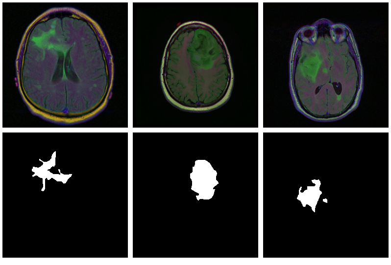
Here are three examples where the masks do indicate
abnormalities:

Let’s see if we can build a U-Net that generates such masks
for us.

Data

Before you start typing, here is a
Colaboratory notebook
to conveniently follow along.

We use pins to obtain the data. Please see this
introduction
if you haven’t used that package before.

# deep learning (incl. dependencies) library(torch) library(torchvision) # data wrangling library(tidyverse) library(zeallot) # image processing and visualization library(magick) library(cowplot) # dataset loading library(pins) library(zip) torch_manual_seed(777) set.seed(777) # use your own kaggle.json here pins::board_register_kaggle(token = "~/kaggle.json") files <- pins::pin_get("mateuszbuda/lgg-mri-segmentation", board = "kaggle", extract = FALSE)

The dataset is not that big – it includes scans from 110
different patients – so we’ll have to do with just a training
and a validation set. (Don’t do this in real life, as you’ll
inevitably end up fine-tuning on the latter.)

train_dir <- "data/mri_train" valid_dir <- "data/mri_valid" if(dir.exists(train_dir)) unlink(train_dir, recursive = TRUE, force = TRUE) if(dir.exists(valid_dir)) unlink(valid_dir, recursive = TRUE, force = TRUE) zip::unzip(files, exdir = "data") file.rename("data/kaggle_3m", train_dir) # this is a duplicate, again containing kaggle_3m (evidently a packaging error on Kaggle) # we just remove it unlink("data/lgg-mri-segmentation", recursive = TRUE) dir.create(valid_dir)

Of those 110 patients, we keep 30 for validation. Some more file
manipulations, and we’re set up with a nice hierarchical
structure, with train_dir and valid_dir holding their per-patient
sub-directories, respectively.

valid_indices <- sample(1:length(patients), 30) patients <- list.dirs(train_dir, recursive = FALSE) for (i in valid_indices) { dir.create(file.path(valid_dir, basename(patients[i]))) for (f in list.files(patients[i])) { file.rename(file.path(train_dir, basename(patients[i]), f), file.path(valid_dir, basename(patients[i]), f)) } unlink(file.path(train_dir, basename(patients[i])), recursive = TRUE) }

We now need a dataset that knows what to do with these
files.

Dataset

Like every torch dataset, this one has initialize() and
.getitem() methods. initialize() creates an inventory of scan and
mask file names, to be used by .getitem() when it actually reads
those files. In contrast to what we’ve seen in previous posts,
though , .getitem() does not simply return input-target pairs in
order. Instead, whenever the parameter random_sampling is true, it
will perform weighted sampling, preferring items with sizable
lesions. This option will be used for the training set, to counter
the class imbalance mentioned above.

The other way training and validation sets will differ is use of
data augmentation. Training images/masks may be flipped, re-sized,
and rotated; probabilities and amounts are configurable.

An instance of brainseg_dataset encapsulates all this
functionality:

brainseg_dataset <- dataset( name = "brainseg_dataset", initialize = function(img_dir, augmentation_params = NULL, random_sampling = FALSE) { self$images <- tibble( img = grep( list.files( img_dir, full.names = TRUE, pattern = "tif", recursive = TRUE ), pattern = 'mask', invert = TRUE, value = TRUE ), mask = grep( list.files( img_dir, full.names = TRUE, pattern = "tif", recursive = TRUE ), pattern = 'mask', value = TRUE ) ) self$slice_weights <- self$calc_slice_weights(self$images$mask) self$augmentation_params <- augmentation_params self$random_sampling <- random_sampling }, .getitem = function(i) { index <- if (self$random_sampling == TRUE) sample(1:self$.length(), 1, prob = self$slice_weights) else i img <- self$images$img[index] %>% image_read() %>% transform_to_tensor() mask <- self$images$mask[index] %>% image_read() %>% transform_to_tensor() %>% transform_rgb_to_grayscale() %>% torch_unsqueeze(1) img <- self$min_max_scale(img) if (!is.null(self$augmentation_params)) { scale_param <- self$augmentation_params[1] c(img, mask) %<-% self$resize(img, mask, scale_param) rot_param <- self$augmentation_params[2] c(img, mask) %<-% self$rotate(img, mask, rot_param) flip_param <- self$augmentation_params[3] c(img, mask) %<-% self$flip(img, mask, flip_param) } list(img = img, mask = mask) }, .length = function() { nrow(self$images) }, calc_slice_weights = function(masks) { weights <- map_dbl(masks, function(m) { img <- as.integer(magick::image_data(image_read(m), channels = "gray")) sum(img / 255) }) sum_weights <- sum(weights) num_weights <- length(weights) weights <- weights %>% map_dbl(function(w) { w <- (w + sum_weights * 0.1 / num_weights) / (sum_weights * 1.1) }) weights }, min_max_scale = function(x) { min = x$min()$item() max = x$max()$item() x$clamp_(min = min, max = max) x$add_(-min)$div_(max - min + 1e-5) x }, resize = function(img, mask, scale_param) { img_size <- dim(img)[2] rnd_scale <- runif(1, 1 - scale_param, 1 + scale_param) img <- transform_resize(img, size = rnd_scale * img_size) mask <- transform_resize(mask, size = rnd_scale * img_size) diff <- dim(img)[2] - img_size if (diff > 0) { top <- ceiling(diff / 2) left <- ceiling(diff / 2) img <- transform_crop(img, top, left, img_size, img_size) mask <- transform_crop(mask, top, left, img_size, img_size) } else { img <- transform_pad(img, padding = -c( ceiling(diff / 2), floor(diff / 2), ceiling(diff / 2), floor(diff / 2) )) mask <- transform_pad(mask, padding = -c( ceiling(diff / 2), floor(diff / 2), ceiling(diff / 2), floor(diff / 2) )) } list(img, mask) }, rotate = function(img, mask, rot_param) { rnd_rot <- runif(1, 1 - rot_param, 1 + rot_param) img <- transform_rotate(img, angle = rnd_rot) mask <- transform_rotate(mask, angle = rnd_rot) list(img, mask) }, flip = function(img, mask, flip_param) { rnd_flip <- runif(1) if (rnd_flip > flip_param) { img <- transform_hflip(img) mask <- transform_hflip(mask) } list(img, mask) } )

After instantiation, we see we have 2977 training pairs and 952
validation pairs, respectively:

train_ds <- brainseg_dataset( train_dir, augmentation_params = c(0.05, 15, 0.5), random_sampling = TRUE ) length(train_ds) # 2977 valid_ds <- brainseg_dataset( valid_dir, augmentation_params = NULL, random_sampling = FALSE ) length(valid_ds) # 952

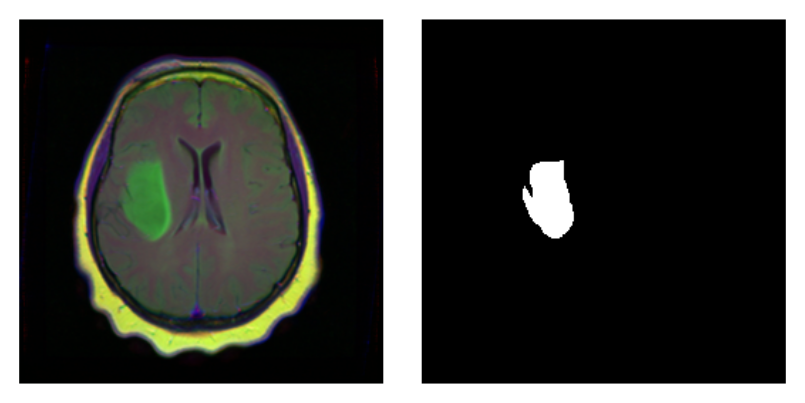
As a correctness check, let’s plot an image and associated
mask:

par(mfrow = c(1, 2), mar = c(0, 1, 0, 1)) img_and_mask <- valid_ds[27] img <- img_and_mask[[1]] mask <- img_and_mask[[2]] img$permute(c(2, 3, 1)) %>% as.array() %>% as.raster() %>% plot() mask$squeeze() %>% as.array() %>% as.raster() %>% plot()

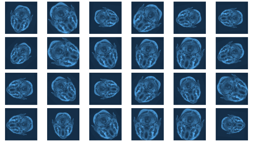
With torch, it is straightforward to inspect what happens when
you change augmentation-related parameters. We just pick a pair
from the validation set, which has not had any augmentation applied
as yet, and call valid_ds$<augmentation_func()> directly.
Just for fun, let’s use more “extreme” parameters here than
we do in actual training. (Actual training uses the settings from
Mateusz’ GitHub repository, which we assume have been carefully
chosen for optimal performance.1)

img_and_mask <- valid_ds[77] img <- img_and_mask[[1]] mask <- img_and_mask[[2]] imgs <- map (1:24, function(i) { # scale factor; train_ds really uses 0.05 c(img, mask) %<-% valid_ds$resize(img, mask, 0.2) c(img, mask) %<-% valid_ds$flip(img, mask, 0.5) # rotation angle; train_ds really uses 15 c(img, mask) %<-% valid_ds$rotate(img, mask, 90) img %>% transform_rgb_to_grayscale() %>% as.array() %>% as_tibble() %>% rowid_to_column(var = "Y") %>% gather(key = "X", value = "value", -Y) %>% mutate(X = as.numeric(gsub("V", "", X))) %>% ggplot(aes(X, Y, fill = value)) + geom_raster() + theme_void() + theme(legend.position = "none") + theme(aspect.ratio = 1) }) plot_grid(plotlist = imgs, nrow = 4)

Now we still need the data loaders, and then, nothing keeps us
from proceeding to the next big task: building the model.

batch_size <- 4 train_dl <- dataloader(train_ds, batch_size) valid_dl <- dataloader(valid_ds, batch_size)

Model

Our model nicely illustrates the kind of modular code that comes
“naturally” with torch. We approach things top-down, starting
with the U-Net container itself.

unet takes care of the global composition – how far “down”
do we go, shrinking the image while incrementing the number of
filters, and then how do we go “up” again?

Importantly, it is also in the system’s memory. In forward(),
it keeps track of layer outputs seen going “down”, to be added
back in going “up”.

unet <- nn_module( "unet", initialize = function(channels_in = 3, n_classes = 1, depth = 5, n_filters = 6) { self$down_path <- nn_module_list() prev_channels <- channels_in for (i in 1:depth) { self$down_path$append(down_block(prev_channels, 2 ^ (n_filters + i - 1))) prev_channels <- 2 ^ (n_filters + i -1) } self$up_path <- nn_module_list() for (i in ((depth - 1):1)) { self$up_path$append(up_block(prev_channels, 2 ^ (n_filters + i - 1))) prev_channels <- 2 ^ (n_filters + i - 1) } self$last = nn_conv2d(prev_channels, n_classes, kernel_size = 1) }, forward = function(x) { blocks <- list() for (i in 1:length(self$down_path)) { x <- self$down_path[[i]](x) if (i != length(self$down_path)) { blocks <- c(blocks, x) x <- nnf_max_pool2d(x, 2) } } for (i in 1:length(self$up_path)) { x <- self$up_path[[i]](x, blocks[[length(blocks) - i + 1]]$to(device = device)) } torch_sigmoid(self$last(x)) } )

unet delegates to two containers just below it in the hierarchy:
down_block and up_block. While down_block is “just” there for
aesthetic reasons (it immediately delegates to its own workhorse,
conv_block), in up_block we see the U-Net “bridges” in
action.

down_block <- nn_module( "down_block", initialize = function(in_size, out_size) { self$conv_block <- conv_block(in_size, out_size) }, forward = function(x) { self$conv_block(x) } ) up_block <- nn_module( "up_block", initialize = function(in_size, out_size) { self$up = nn_conv_transpose2d(in_size, out_size, kernel_size = 2, stride = 2) self$conv_block = conv_block(in_size, out_size) }, forward = function(x, bridge) { up <- self$up(x) torch_cat(list(up, bridge), 2) %>% self$conv_block() } )

Finally, a conv_block is a sequential structure containing
convolutional, ReLU, and dropout layers.

conv_block <- nn_module( "conv_block", initialize = function(in_size, out_size) { self$conv_block <- nn_sequential( nn_conv2d(in_size, out_size, kernel_size = 3, padding = 1), nn_relu(), nn_dropout(0.6), nn_conv2d(out_size, out_size, kernel_size = 3, padding = 1), nn_relu() ) }, forward = function(x){ self$conv_block(x) } )

Now instantiate the model, and possibly, move it to the GPU:

device <- torch_device(if(cuda_is_available()) "cuda" else "cpu") model <- unet(depth = 5)$to(device = device)

Optimization

We train our model with a combination of cross entropy and

dice loss
.

The latter, though not shipped with torch, may be implemented
manually:

calc_dice_loss <- function(y_pred, y_true) { smooth <- 1 y_pred <- y_pred$view(-1) y_true <- y_true$view(-1) intersection <- (y_pred * y_true)$sum() 1 - ((2 * intersection + smooth) / (y_pred$sum() + y_true$sum() + smooth)) } dice_weight <- 0.3

Optimization uses stochastic gradient descent (SGD), together
with the one-cycle learning rate scheduler introduced in the
context of
image classification with torch
.

optimizer <- optim_sgd(model$parameters, lr = 0.1, momentum = 0.9) num_epochs <- 20 scheduler <- lr_one_cycle( optimizer, max_lr = 0.1, steps_per_epoch = length(train_dl), epochs = num_epochs )

Training

The training loop then follows the usual scheme. One thing to
note: Every epoch, we save the model (using torch_save()), so we
can later pick the best one, should performance have degraded
thereafter.

train_batch <- function(b) { optimizer$zero_grad() output <- model(b[[1]]$to(device = device)) target <- b[[2]]$to(device = device) bce_loss <- nnf_binary_cross_entropy(output, target) dice_loss <- calc_dice_loss(output, target) loss <- dice_weight * dice_loss + (1 - dice_weight) * bce_loss loss$backward() optimizer$step() scheduler$step() list(bce_loss$item(), dice_loss$item(), loss$item()) } valid_batch <- function(b) { output <- model(b[[1]]$to(device = device)) target <- b[[2]]$to(device = device) bce_loss <- nnf_binary_cross_entropy(output, target) dice_loss <- calc_dice_loss(output, target) loss <- dice_weight * dice_loss + (1 - dice_weight) * bce_loss list(bce_loss$item(), dice_loss$item(), loss$item()) } for (epoch in 1:num_epochs) { model$train() train_bce <- c() train_dice <- c() train_loss <- c() for (b in enumerate(train_dl)) { c(bce_loss, dice_loss, loss) %<-% train_batch(b) train_bce <- c(train_bce, bce_loss) train_dice <- c(train_dice, dice_loss) train_loss <- c(train_loss, loss) } torch_save(model, paste0("model_", epoch, ".pt")) cat(sprintf("nEpoch %d, training: loss:%3f, bce: %3f, dice: %3fn", epoch, mean(train_loss), mean(train_bce), mean(train_dice))) model$eval() valid_bce <- c() valid_dice <- c() valid_loss <- c() i <- 0 for (b in enumerate(valid_dl)) { i <<- i + 1 c(bce_loss, dice_loss, loss) %<-% valid_batch(b) valid_bce <- c(valid_bce, bce_loss) valid_dice <- c(valid_dice, dice_loss) valid_loss <- c(valid_loss, loss) } cat(sprintf("nEpoch %d, validation: loss:%3f, bce: %3f, dice: %3fn", epoch, mean(valid_loss), mean(valid_bce), mean(valid_dice))) }
Epoch 1, training: loss:0.304232, bce: 0.148578, dice: 0.667423 Epoch 1, validation: loss:0.333961, bce: 0.127171, dice: 0.816471 Epoch 2, training: loss:0.194665, bce: 0.101973, dice: 0.410945 Epoch 2, validation: loss:0.341121, bce: 0.117465, dice: 0.862983 [...] Epoch 19, training: loss:0.073863, bce: 0.038559, dice: 0.156236 Epoch 19, validation: loss:0.302878, bce: 0.109721, dice: 0.753577 Epoch 20, training: loss:0.070621, bce: 0.036578, dice: 0.150055 Epoch 20, validation: loss:0.295852, bce: 0.101750, dice: 0.748757

Evaluation

In this run, it is the final model that performs best on the
validation set. Still, we’d like to show how to load a saved
model, using torch_load() .

Once loaded, put the model into eval mode:

saved_model <- torch_load("model_20.pt") model <- saved_model model$eval()

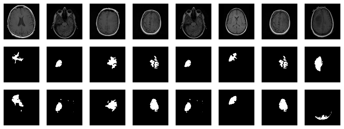
Now, since we don’t have a separate test set, we already know
the average out-of-sample metrics; but in the end, what we care
about are the generated masks. Let’s view some, displaying ground
truth and MRI scans for comparison.

# without random sampling, we'd mainly see lesion-free patches eval_ds <- brainseg_dataset(valid_dir, augmentation_params = NULL, random_sampling = TRUE) eval_dl <- dataloader(eval_ds, batch_size = 8) batch <- eval_dl %>% dataloader_make_iter() %>% dataloader_next() par(mfcol = c(3, 8), mar = c(0, 1, 0, 1)) for (i in 1:8) { img <- batch[[1]][i, .., drop = FALSE] inferred_mask <- model(img$to(device = device)) true_mask <- batch[[2]][i, .., drop = FALSE]$to(device = device) bce <- nnf_binary_cross_entropy(inferred_mask, true_mask)$to(device = "cpu") %>% as.numeric() dc <- calc_dice_loss(inferred_mask, true_mask)$to(device = "cpu") %>% as.numeric() cat(sprintf("nSample %d, bce: %3f, dice: %3fn", i, bce, dc)) inferred_mask <- inferred_mask$to(device = "cpu") %>% as.array() %>% .[1, 1, , ] inferred_mask <- ifelse(inferred_mask > 0.5, 1, 0) img[1, 1, ,] %>% as.array() %>% as.raster() %>% plot() true_mask$to(device = "cpu")[1, 1, ,] %>% as.array() %>% as.raster() %>% plot() inferred_mask %>% as.raster() %>% plot() }

We also print the individual cross entropy and dice losses;
relating those to the generated masks might yield useful
information for model tuning.

Sample 1, bce: 0.088406, dice: 0.387786} Sample 2, bce: 0.026839, dice: 0.205724 Sample 3, bce: 0.042575, dice: 0.187884 Sample 4, bce: 0.094989, dice: 0.273895 Sample 5, bce: 0.026839, dice: 0.205724 Sample 6, bce: 0.020917, dice: 0.139484 Sample 7, bce: 0.094989, dice: 0.273895 Sample 8, bce: 2.310956, dice: 0.999824

While far from perfect, most of these masks aren’t that bad
– a nice result given the small dataset!

Wrapup

This has been our most complex torch post so far; however, we
hope you’ve found the time well spent. For one, among
applications of deep learning, medical image segmentation stands
out as highly societally useful. Secondly, U-Net-like architectures
are employed in many other areas. And finally, we once more saw
torch’s flexibility and intuitive behavior in action.

Thanks for reading!

Buda, Mateusz, Ashirbani Saha, and Maciej A. Mazurowski. 2019.
“Association of Genomic Subtypes of Lower-Grade Gliomas with
Shape Features Automatically Extracted by a Deep Learning
Algorithm.” Computers in Biology and Medicine 109: 218–25.
https://doi.org/https://doi.org/10.1016/j.compbiomed.2019.05.002.

Ronneberger, Olaf, Philipp Fischer, and Thomas Brox. 2015.
“U-Net: Convolutional Networks for Biomedical Image
Segmentation.” CoRR abs/1505.04597. http://arxiv.org/abs/1505.04597.

  1. Yes, we did a few experiments, confirming that more augmentation
    isn’t better … what did I say about inevitably ending up doing
    optimization on the validation set …?↩︎

Categories
Misc

Python TensorFlow Tutorial – Build a Neural Network

Updated for TensorFlow 2

Google’s TensorFlow has been a hot topic in deep learning
recently. The open source software, designed to allow efficient
computation of data flow graphs, is especially suited to deep
learning tasks. It is designed to be executed on single or
multiple CPUs and GPUs, making it a good option for complex deep
learning tasks.  In its most recent incarnation – version 1.0 –
it can even be run on certain mobile operating systems.  This
introductory tutorial to TensorFlow will give an overview of some
of the basic concepts of TensorFlow in Python.  These will be a
good stepping stone to building more complex deep learning
networks, such as
Convolution Neural Networks
,
natural language models
, and
Recurrent Neural Networks
in the package.  We’ll be creating a
simple three-layer neural network to classify the MNIST dataset. 
This tutorial assumes that you are familiar with the basics of
neural networks, which you can get up to scratch with in the

neural networks tutorial
if required.  To install TensorFlow,
follow the instructions here. The code for this
tutorial can be found in this
site’s GitHub repository
.  Once you’re done, you also might
want to check out a higher level deep learning library that sits on
top of TensorFlow called Keras – see
my Keras tutorial
.

First, let’s have a look at the main ideas of TensorFlow.

1.0 TensorFlow graphs

TensorFlow is based on graph based computation – “what on
earth is that?”, you might say.  It’s an alternative way
of conceptualising mathematical calculations.  Consider the
following expression $a = (b + c) * (c + 2)$.  We can break this
function down into the following components:

begin{align}
d &= b + c \
e &= c + 2 \
a &= d * e
end{align}

Now we can represent these operations graphically as:

TensorFlow tutorial - simple computational graph

Simple computational graph

This may seem like a silly example – but notice a powerful
idea in expressing the equation this way: two of the computations
($d=b+c$ and $e=c+2$) can be performed in parallel.  By splitting
up these calculations across CPUs or GPUs, this can give us
significant gains in computational times.  These gains are a must
for big data applications and deep learning – especially for
complicated neural network architectures such as Convolutional
Neural Networks (CNNs) and Recurrent Neural Networks (RNNs).  The
idea behind TensorFlow is to the ability to create these
computational graphs in code and allow significant performance
improvements via parallel operations and other efficiency
gains.

We can look at a similar graph in TensorFlow below, which shows
the computational graph of a three-layer neural network.

TensorFlow tutorial - data flow graph

TensorFlow data flow graph

The animated data flows between different nodes in the graph are
tensors which are multi-dimensional data arrays.  For instance, the
input data tensor may be 5000 x 64 x 1, which represents a 64 node
input layer with 5000 training samples.  After the input layer,
there is a hidden layer with rectified
linear units
as the activation function.  There is a final
output layer (called a “logit layer” in the above graph) that
uses cross-entropy as a cost/loss function.  At each point we see
the relevant tensors flowing to the “Gradients” block which
finally flows to the
Stochastic Gradient Descent
optimizer which performs the
back-propagation and gradient descent.

Here we can see how computational graphs can be used to
represent the calculations in neural networks, and this, of course,
is what TensorFlow excels at.  Let’s see how to perform some basic
mathematical operations in TensorFlow to get a feel for how it all
works.

2.0 A Simple TensorFlow example

So how can we make TensorFlow perform the little example
calculation shown above – $a = (b + c) * (c + 2)$? First, there
is a need to introduce TensorFlow variables.  The code below shows
how to declare these objects:

import tensorflow as tf
# create TensorFlow variables
const = tf.Variable(2.0, name="const")
b = tf.Variable(2.0, name='b')
c = tf.Variable(1.0, name='c')

As can be observed above, TensorFlow variables can be declared
using the tf.Variable function.  The first argument is the value to
be assigned to the variable. The second is an optional name string
which can be used to label the constant/variable – this is handy
for when you want to do visualizations.  TensorFlow will infer the
type of the variable from the initialized value, but it can also be
set explicitly using the optional dtype argument.  TensorFlow has
many of its own types like tf.float32, tf.int32 etc.

The objects assigned to the Python variables are actually
TensorFlow tensors. Thereafter, they act like normal Python objects
– therefore, if you want to access the tensors you need to keep
track of the Python variables. In previous versions of TensorFlow,
there were global methods of accessing the tensors and operations
based on their names. This is no longer the case.

To examine the tensors stored in the Python variables, simply
call them as you would a normal Python variable. If we do this for
the “const” variable, you will see the following output:

<tf.Variable ‘const:0′ shape=() dtype=float32,
numpy=2.0>

This output gives you a few different pieces of information –
first, is the name ‘const:0’ which has been assigned to the
tensor. Next is the data type, in this case, a TensorFlow float 32
type. Finally, there is a “numpy” value. TensorFlow variables
in TensorFlow 2 can be converted easily into numpy objects. Numpy
stands for Numerical Python and is a crucial library for Python
data science and machine learning. If you don’t know Numpy, what
it is, and how to use it, check out this site. The command to access the
numpy form of the tensor is simply .numpy() – the use of this
method will be shown shortly.

Next, some calculation operations are created:

# now create some operations
d = tf.add(b, c, name='d')
e = tf.add(c, const, name='e')
a = tf.multiply(d, e, name='a')

Note that d and e are automatically converted to tensor values
upon the execution of the operations. TensorFlow has a wealth of
calculation operations available to perform all sorts of
interactions between tensors, as you will discover as you progress
through this book.  The purpose of the operations shown above are
pretty obvious, and they instantiate the operations b + c, c + 2.0,
and d * e. However, these operations are an unwieldy way of doing
things in TensorFlow 2. The operations below are equivalent to
those above:

d = b + c
e = c + 2
a = d * e

To access the value of variable a, one can use the .numpy()
method as shown below:

print(f”Variable a is {a.numpy()}”)

The computational graph for this simple example can be
visualized by using the TensorBoard functionality that comes
packaged with TensorFlow. This is a great visualization feature and
is explained more in
this post
. Here is what the graph looks like in
TensorBoard:

TensorFlow tutorial - simple graph

Simple TensorFlow graph

The larger two vertices or nodes, b and c, correspond to the
variables. The smaller nodes correspond to the operations, and the
edges between the vertices are the scalar values emerging from the
variables and operations.

The example above is a trivial example – what would this look
like if there was an array of b values from which an array of
equivalent a values would be calculated? TensorFlow variables can
easily be instantiated using numpy variables, like the
following:

b = tf.Variable(np.arange(0, 10), name='b')

Calling b shows the following:

<tf.Variable ‘b:0′ shape=(10,) dtype=int32, numpy=array([0,
1, 2, 3, 4, 5, 6, 7, 8, 9])>

Note the numpy value of the tensor is an array. Because the
numpy variable passed during the instantiation is a range of int32
values, we can’t add it directly to c as c is of float32 type.
Therefore, the tf.cast operation, which changes the type of a
tensor, first needs to be utilized like so:

d = tf.cast(b, tf.float32) + c

Running the rest of the previous operations, using the new b
tensor, gives the following value for a:

Variable a is [ 3.  6.  9. 12. 15. 18. 21. 24. 27. 30.]

In numpy, the developer can directly access slices or individual
indices of an array and change their values directly. Can the same
be done in TensorFlow 2? Can individual indices and/or slices be
accessed and changed? The answer is yes, but not quite as
straight-forwardly as in numpy. For instance, if b was a simple
numpy array, one could easily execute the following b[1] = 10 –
this would change the value of the second element in the array to
the integer 10.

b[1].assign(10)

This will then flow through to a like so:

Variable a is [ 3. 33.  9. 12. 15. 18. 21. 24. 27. 30.]

The developer could also run the following, to assign a slice of
b values:

b[6:9].assign([10, 10, 10])

A new tensor can also be created by using the slice
notation:

f = b[2:5]

The explanations and code above show you how to perform some
basic tensor manipulations and operations. In the section below, an
example will be presented where a neural network is created using
the Eager paradigm in TensorFlow 2. It will show how to create a
training loop, perform a feed-forward pass through a neural network
and calculate and apply gradients to an optimization method.

3.0 A Neural Network Example

In this section, a simple three-layer neural network build in
TensorFlow is demonstrated.  In following chapters more complicated
neural network structures such as convolution neural networks and
recurrent neural networks are covered.  For this example, though,
it will be kept simple.

In this example, the MNIST dataset will be used that is packaged
as part of the TensorFlow installation. This MNIST dataset is a set
of 28×28 pixel grayscale images which represent hand-written
digits.  It has 60,000 training rows, 10,000 testing rows, and
5,000 validation rows. It is a very common, basic, image
classification dataset that is used in machine learning.

The data can be loaded by running the following:

from tensorflow.keras.datasets import mnist
(x_train, y_train), (x_test, y_test) = mnist.load_data()

As can be observed, the Keras MNIST data loader returns Python
tuples corresponding to the training and test set respectively
(Keras is another deep learning framework, now tightly integrated
with TensorFlow, as mentioned earlier). The data sizes of the
tuples defined above are:

  • x_train: (60,000 x 28 x 28)
  • y_train: (60,000)
  • x_test: (10,000 x 28 x 28)
  • y_test: (10,000)

The x data is the image information – 60,000 images of 28 x 28
pixels size in the training set. The images are grayscale (i.e
black and white) with maximum values, specifying the intensity of
whites, of 255. The x data will need to be scaled so that it
resides between 0 and 1, as this improves training efficiency. The
y data is the matching image labels – signifying what digit is
displayed in the image. This will need to be transformed to
“one-hot” format.

When using a standard, categorical cross-entropy loss function
(this will be shown later), a one-hot format is required when
training classification tasks, as the output layer of the neural
network will have the same number of nodes as the total number of
possible classification labels. The output node with the highest
value is considered as a prediction for that corresponding label.
For instance, in the MNIST task, there are 10 possible
classification labels – 0 to 9. Therefore, there will be 10
output nodes in any neural network performing this classification
task. If we have an example output vector of [0.01, 0.8, 0.25,
0.05, 0.10, 0.27, 0.55, 0.32, 0.11, 0.09], the maximum value is in
the second position / output node, and therefore this corresponds
to the digit “1”. To train the network to produce this sort of
outcome when the digit “1” appears, the loss needs to be
calculated according to the difference between the output of the
network and a “one-hot” array of the label 1. This one-hot
array looks like [0, 1, 0, 0, 0, 0, 0, 0, 0, 0].

This conversion is easily performed in TensorFlow, as will be
demonstrated shortly when the main training loop is covered.

One final thing that needs to be considered is how to extract
the training data in batches of samples. The function below can
handle this:

def get_batch(x_data, y_data, batch_size):
    idxs = np.random.randint(0, len(y_data), batch_size)
    return x_data[idxs,:,:], y_data[idxs]

As can be observed in the code above, the data to be batched
i.e. the x and y data is passed to this function along with the
batch size. The first line of the function generates a random
vector of integers, with random values between 0 and the length of
the data passed to the function. The number of random integers
generated is equal to the batch size. The x and y data are then
returned, but the return data is only for those random indices
chosen. Note, that this is performed on numpy array objects – as
will be shown shortly, the conversion from numpy arrays to tensor
objects will be performed “on the fly” within the training
loop.

There is also the requirement for a loss function and a
feed-forward function, but these will be covered shortly.

# Python optimisation variables
epochs = 10
batch_size = 100

# normalize the input images by dividing by 255.0
x_train = x_train / 255.0
x_test = x_test / 255.0
# convert x_test to tensor to pass through model (train data will be converted to
# tensors on the fly)
x_test = tf.Variable(x_test)

First, the number of training epochs and the batch size are
created – note these are simple Python variables, not TensorFlow
variables. Next, the input training and test data, x_train and
x_test, are scaled so that their values are between 0 and 1. Input
data should always be scaled when training neural networks, as
large, uncontrolled, inputs can heavily impact the training
process. Finally, the test input data, x_test is converted into a
tensor. The random batching process for the training data is most
easily performed using numpy objects and functions. However, the
test data will not be batched in this example, so the full test
input data set x_test is converted into a tensor.

The next step is to setup the weight and bias variables for the
three-layer neural network.  There are always L – 1 number of
weights/bias tensors, where L is the number of layers.  These
variables are defined in the code below:

# now declare the weights connecting the input to the hidden layer
W1 = tf.Variable(tf.random.normal([784, 300], stddev=0.03), name='W1')
b1 = tf.Variable(tf.random.normal([300]), name='b1')
# and the weights connecting the hidden layer to the output layer
W2 = tf.Variable(tf.random.normal([300, 10], stddev=0.03), name='W2')
b2 = tf.Variable(tf.random.normal([10]), name='b2')

The weight and bias variables are initialized using the
tf.random.normal function – this function creates tensors of
random numbers, drawn from a normal distribution. It allows the
developer to specify things like the standard deviation of the
distribution from which the random numbers are drawn.

Note the shape of the variables. The W1 variable is a [784, 300]
tensor – the 784 nodes are the size of the input layer. This size
comes from the flattening of the input images – if we have 28
rows and 28 columns of pixels, flattening these out gives us 1 row
or column of 28 x 28 = 784 values.  The 300 in the declaration of
W1 is the number of nodes in the hidden layer. The W2 variable is a
[300, 10] tensor, connecting the 300-node hidden layer to the
10-node output layer. In each case, a name is given to the variable
for later viewing in TensorBoard – the TensorFlow visualization
package. The next step in the code is to create the computations
that occur within the nodes of the network. If the reader recalls,
the computations within the nodes of a neural network are of the
following form:

$$z = Wx + b$$

$$h=f(z)$$

Where W is the weights matrix, x is the layer input vector, b is
the bias and f is the activation function of the node. These
calculations comprise the feed-forward pass of the input data
through the neural network. To execute these calculations, a
dedicated feed-forward function is created:

def nn_model(x_input, W1, b1, W2, b2):
    # flatten the input image from 28 x 28 to 784
    x_input = tf.reshape(x_input, (x_input.shape[0], -1))
    x = tf.add(tf.matmul(tf.cast(x_input, tf.float32), W1), b1)
    x = tf.nn.relu(x)
    logits = tf.add(tf.matmul(x, W2), b2)
    return logits

Examining the first line, the x_input data is reshaped from
(batch_size, 28, 28) to (batch_size, 784) – in other words, the
images are flattened out. On the next line, the input data is then
converted to tf.float32 type using the TensorFlow cast function.
This is important – the x­_input data comes in as tf.float64
type, and TensorFlow won’t perform a matrix multiplication
operation (tf.matmul) between tensors of different data types. This
re-typed input data is then matrix-multiplied by W1 using the
TensorFlow matmul function (which stands for matrix
multiplication). Then the bias b1 is added to this product. On the
line after this, the ReLU activation function is applied to the
output of this line of calculation. The ReLU function is usually
the best activation function to use in deep learning – the
reasons for this are discussed in
this post
.

The output of this calculation is then multiplied by the final
set of weights W2, with the bias b2 added. The output of this
calculation is titled logits. Note that no activation function has
been applied to this output layer of nodes (yet). In machine/deep
learning, the term “logits” refers to the un-activated output
of a layer of nodes.

The reason no activation function has been applied to this layer
is that there is a handy function in TensorFlow called
tf.nn.softmax_cross_entropy_with_logits. This function does two
things for the developer – it applies a softmax activation
function to the logits, which transforms them into a
quasi-probability (i.e. the sum of the output nodes is equal to 1).
This is a common activation function to apply to an output layer in
classification tasks. Next, it applies the cross-entropy loss
function to the softmax activation output. The cross-entropy loss
function is a commonly used loss in classification tasks. The
theory behind it is quite interesting, but it won’t be covered in
this book – a good summary can be found
here
. The code below applies this handy TensorFlow function,
and in this example,  it has been nested in another function called
loss_fn:

def loss_fn(logits, labels):
    cross_entropy = tf.reduce_mean(tf.nn.softmax_cross_entropy_with_logits(labels=labels,
                                                                              logits=logits))
    return cross_entropy

The arguments to softmax_cross_entropy_with_logits are labels
and logits. The logits argument is supplied from the outcome of the
nn_model function. The usage of this function in the main training
loop will be demonstrated shortly. The labels argument is supplied
from the one-hot y values that are fed into loss_fn during the
training process. The output of the
softmax_cross_entropy_with_logits function will be the output of
the cross-entropy loss value for each sample in the batch. To train
the weights of the neural network, the average cross-entropy loss
across the samples needs to be minimized as part of the
optimization process. This is calculated by using the
tf.reduce_mean function, which, unsurprisingly, calculates the mean
of the tensor supplied to it.

The next step is to define an optimizer function. In many
examples within this book, the versatile Adam optimizer will be
used. The theory behind this optimizer is interesting, and is worth
further examination (such as shown here)
but won’t be covered in detail within this post. It is basically
a gradient descent method, but with sophisticated averaging of the
gradients to provide appropriate momentum to the learning. To
define the optimizer, which will be used in the main training loop,
the following code is run:

# setup the optimizer
optimizer = tf.keras.optimizers.Adam()

The Adam object can take a learning rate as input, but for the
present purposes, the default value is used.

3.1 Training the network

Now that the appropriate functions, variables and optimizers
have been created, it is time to define the overall training loop.
The training loop is shown below:

total_batch = int(len(y_train) / batch_size)
for epoch in range(epochs):
    avg_loss = 0
    for i in range(total_batch):
        batch_x, batch_y = get_batch(x_train, y_train, batch_size=batch_size)
        # create tensors
        batch_x = tf.Variable(batch_x)
        batch_y =..
Categories
Misc

Inserting layers in existing pre-trained model

I’m trying out transfer learning for the first time and I’m
wondering if I can insert layers into the existing model. And is it
possible to change some of the layers of the pre-trained, for
example adding regularization to some of the existing layers.
Thanks in advance!

submitted by /u/ThomaschOmatic

[visit reddit]

[comments]

Categories
Misc

How to stop CUDA from re-initializing for every subprocess which trains a keras model?

I am using CUDA/CUDNN to train multiple tensorflow keras models
on my GPU (for an evolutionary algorithm attempting to optimize
hyperparameters). Initially, the program would crash with an Out of
Memory error after a couple generations. Eventually, I found that
using a new sub-process for every model would clear the GPU memory
automatically.

However, each process seems to reinitialize CUDA (loading
dynamic libraries from the .dll files), which is incredibly
time-consuming. Is there any method to avoid this?

Code is pasted below. The function “fitness_wrapper” is called
for each individual.

def fitness_wrapper(indiv): fit = multi.processing.Value('d', 0.0) if __name__ == '__main__': process = multiprocessing.Process(target=fitness, args=(indiv, fit)) process.start() process.join() return (fit.value,) def fitness(indiv, fit): model = tf.keras.Sequential.from_config(indiv['architecture']) optimizer_dict = indiv['optimizer'] opt = tf.keras.optimizers.Adam(learning_rate=optimizer_dict['lr'], beta_1=optimizer_dict['b1'], beta_2=optimizer_dict['b2'], epsilon=optimizer_dict['epsilon']) model.compile(loss='binary_crossentropy', optimizer=opt, metrics=['accuracy']) model.fit(data_split[0], data_split[2], batch_size=32, epochs=5) fit = model.evaluate(data_split[1], data_split[3])[1] 

submitted by /u/BadassGhost

[visit reddit]

[comments]

Categories
Misc

Chalk and Awe: Studio Crafts Creative Battle Between Stick Figures with Real-Time Rendering

It’s time to bring krisp graphics to stick figure drawings. Creative studio SoKrispyMedia, started by content creators Sam Wickert and Eric Leigh, develops short videos blended with high-quality visual effects. Since publishing one of their early works eight years ago on YouTube, Chalk Warfare 1, the team has regularly put out short films that showcase Read article >

The post Chalk and Awe: Studio Crafts Creative Battle Between Stick Figures with Real-Time Rendering appeared first on The Official NVIDIA Blog.

Categories
Misc

Big Wheels Keep on Learnin’: Einride’s AI Trucks Advance Capabilities with NVIDIA DRIVE AGX Orin

Swedish startup Einride has rejigged the big rig for highways around the world. The autonomous truck maker launched the next generation of its cab-less autonomous truck, known as the Pod, with new, advanced functionality and pricing. The AI vehicles, which will be commercially available worldwide, will be powered by the latest in high-performance, energy-efficient compute Read article >

The post Big Wheels Keep on Learnin’: Einride’s AI Trucks Advance Capabilities with NVIDIA DRIVE AGX Orin appeared first on The Official NVIDIA Blog.

Categories
Misc

NVIDIA Boosts Academic AI Research for Business Innovation

Academic researchers are developing AI to solve challenging problems with everything from agricultural robotics to autonomous flying machines. To help AI research like this make the leap from academia to commercial or government deployment, NVIDIA today announced the Applied Research Accelerator Program. The program supports applied research on NVIDIA platforms for GPU-accelerated application deployments. The Read article >

The post NVIDIA Boosts Academic AI Research for Business Innovation appeared first on The Official NVIDIA Blog.

Categories
Misc

NVIDIA Research Achieves AI Training Breakthrough Using Limited Datasets

NVIDIA Research’s latest AI model is a prodigy among generative adversarial networks. Using a fraction of the study material needed by a typical GAN, it can learn skills as complex as emulating renowned painters and recreating images of cancer tissue. By applying a breakthrough neural network training technique to the popular NVIDIA StyleGAN2 model, NVIDIA Read article >

The post NVIDIA Research Achieves AI Training Breakthrough Using Limited Datasets appeared first on The Official NVIDIA Blog.